How Much Is One Recurrence Worth? Iso-Depth Scaling Laws for Looped Language Models
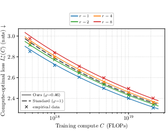
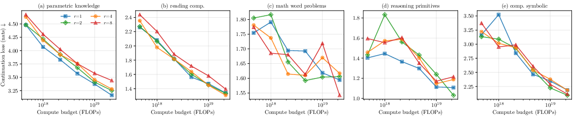
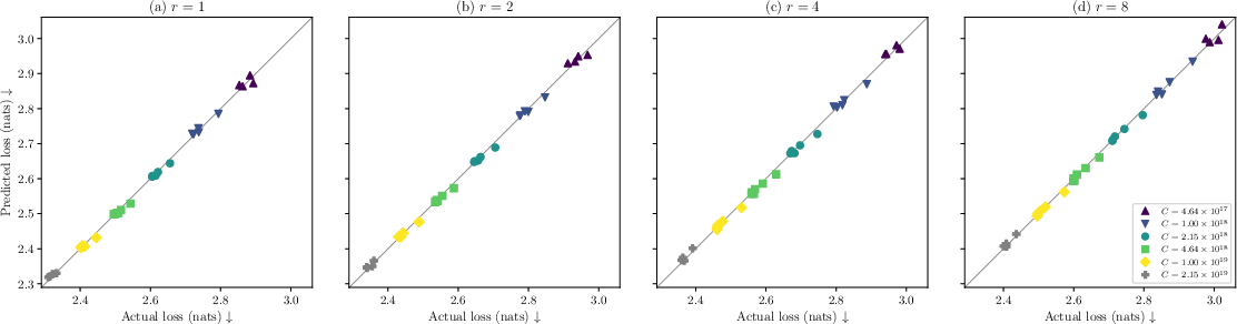
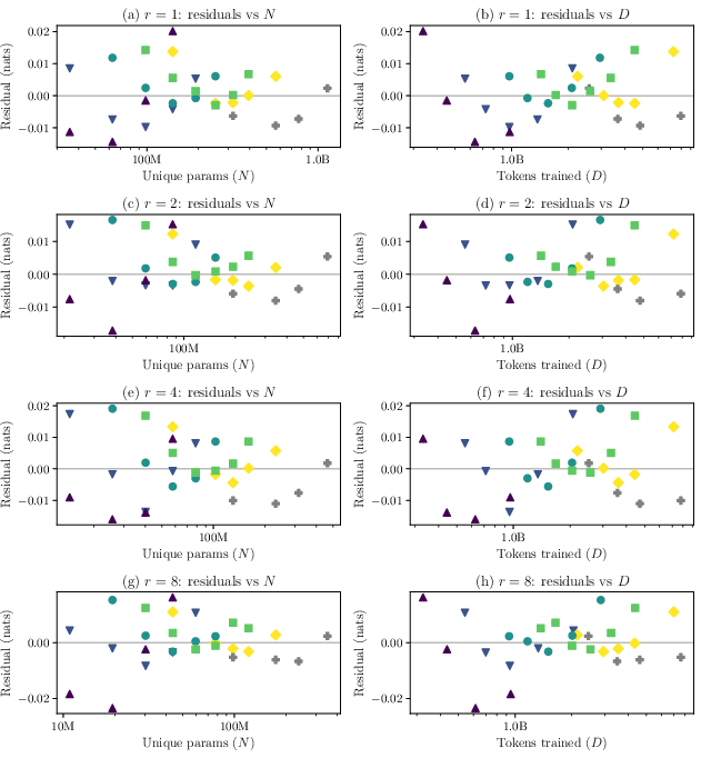
Abstract: We measure how much one extra recurrence is worth to a looped (depth-recurrent) LLM, in equivalent unique parameters. From an iso-depth sweep of 116 pretraining runs across recurrence counts $r \in {1, 2, 4, 8}$ spanning ${\sim}50\times$ in training compute, we fit a joint scaling law $L = E + A\,(N_\text{once} + r{\varphi} N_\text{rec}){-α} + B\,D{-β}$ and recover a new recurrence-equivalence exponent $\varphi = 0.46$ at $R2 = 0.997$. Intuitively, $\varphi$ tells us whether looping a block $r$ times is equivalent in validation loss to $r$ unique blocks of a non-looped model (full equivalence, $\varphi{=}1$) or to a single block run repeatedly with no capacity gain ($\varphi{=}0$). Our $\varphi = 0.46$ sits in between, so each additional recurrence predictably increases validation loss at matched training compute. For example, at $r{=}4$ a 410M looped model performs on par with a 580M non-looped model, but pays the training cost of a 1B non-looped one. On a five-axis downstream evaluation, the gap persists on parametric-knowledge tasks and closes on simple open-book tasks, while reasoning tasks are not resolvable at our compute budgets. For any looped LM, our $\varphi$ converts the design choice of $r$ into a predictable validation-loss cost, and future training recipes and architectures can be compared by how much they raise $\varphi$ above $0.46$.
Paper Prompts
Sign up for free to create and run prompts on this paper using GPT-5.
Top Community Prompts
Explain it Like I'm 14
Overview: What this paper is about
This paper studies a simple question about “looped” LMs: if you reuse the same set of layers multiple times (loop them) instead of building many different layers, how much does each extra loop help? The authors measure this in a fair way and create a formula that tells you how valuable one more loop is, compared to adding a brand‑new layer.
The key questions in plain language
- If you repeat the same block of layers times (looping), is that just as good as having different blocks (no sharing) when you spend the same amount of computing power?
- How can we put a single number on “how much a loop is worth” so that different model designs can be compared easily?
- Where does the benefit or cost of looping show up: in memorized knowledge, reading and extraction, or reasoning tasks?
How they tested it (methods, with simple analogies)
Think of building a tower out of LEGO:
- A non-looped model is like stacking 20 different LEGO floors (each floor is unique).
- A looped model is like building fewer unique floors but walking around each floor multiple times (looping it) to do more work with the same pieces.
The authors made four versions of the same “height” (effective depth) of model:
- (no looping, baseline),
- , , and (looping the shared block 2, 4, or 8 times).
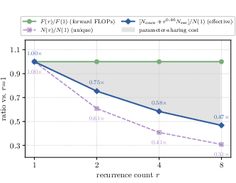
They kept the total number of steps the model takes per token the same across all versions, so each token costs about the same compute to process (this is called “iso-depth” and “matched per-token FLOPs”). But the looped versions have fewer unique parameters (fewer unique LEGO floors) because some are reused.
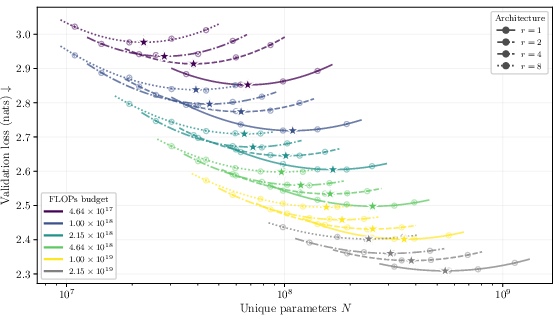
They trained 116 models across six different “compute budgets” (how much total work they let the training do) to find the best settings for each architecture. Then they fit a “scaling law,” which is just a math formula that predicts validation loss (how well the model predicts text) from:
- how many unique parameters the model has,
- how many training tokens it sees,
- and how many times the shared block is looped ().
To capture “how much a loop is worth,” they introduced a new exponent, (phi), in the formula. You can think of like this:
- If , looping times is as good as having different new blocks (full value).
- If , looping adds no value beyond reusing the same block (no extra capacity).
- If , looping helps, but less than adding the same number of new blocks.
They also tested the trained models on different types of tasks (like recalling facts, reading comprehension, and reasoning) to see where looping helps or hurts.
What they found and why it matters
Here are the main results, explained simply:
- The “worth” of a loop is only partial: They measured (very high fit quality, ). That means each extra loop helps, but much less than adding a brand‑new block. For example, looping a block 4 times () acts like about new blocks—not 4.
- A concrete example: At , a looped model with about 410 million parameters performs like a non‑looped model with ~580 million parameters—but it costs as much training compute as training a ~1 billion parameter non‑looped model. So you trade fewer unique parameters for more training work per parameter, and that doesn’t fully pay off.
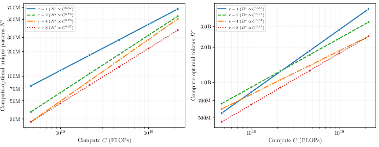
- Best training settings shift when you loop: When you let the training find the best setup at each compute budget, looped models prefer to be wider (more channels per layer) and to see fewer total training tokens. This is useful guidance for training looped LMs.
- Downstream tasks show three patterns:
- Parametric knowledge (closed‑book facts) suffers the most with more looping. This matches the idea that fewer unique parameters means less capacity to store facts.
- Simple open‑book or extraction tasks catch up as overall model quality improves; the gap between looped and non‑looped models shrinks here.
- Reasoning tasks (like multi‑step math or logic probes) don’t show clear, reliable differences at the small‑to‑mid compute sizes used in this study—any advantage is too small to measure at this scale.
Why this matters:
- The single number gives an easy, predictable way to convert “how many loops” into a performance cost or benefit. It turns a design choice (how much you loop) into a clear tradeoff in validation loss.
- The result () sets a baseline. Future training tricks or architecture changes can be judged by whether they raise (make loops “worth more”).
What this means going forward
- Practical design takeaway: At the scales tested, simply looping more isn’t as good as adding new blocks if your goal is the lowest validation loss for the same amount of training compute. If you do choose looping (for memory or deployment reasons), plan for wider layers and fewer training tokens, and expect a performance gap—especially on tasks that rely on memorized knowledge.
- A clear benchmark for improvement: Because measures loop value, new ideas—like cheaper training of each loop (e.g., truncated backprop), adaptive loops that exit early on easy tokens, or retrofitting—can be compared by how much they raise above 0.46.
- What to measure at this scale: Validation loss is the most reliable signal. Many reasoning benchmarks are too hard for small models to show clear differences. So, if you’re developing looped LMs at modest budgets, focusing on closing the validation‑loss gap is the most measurable goal.
- Limits to keep in mind: The study fixed the effective depth (20 layers) and used one common looped design (“prelude–recur–coda”) across , and covered about a 50× range in compute. Results might shift at much larger scales or with different depth layouts, but within this setup, the conclusions are consistent.
In short: looping a shared block helps, but not as much as adding new blocks. The paper gives a clean, predictive rule for that tradeoff, and a simple score () future methods can try to improve.
Knowledge Gaps
Knowledge gaps, limitations, and open questions
Below is a concise, actionable list of what remains uncertain or unexplored in the paper and where future research could extend or stress‐test the findings.
- Scale dependence of φ: The recurrence-equivalence exponent is estimated at development-scale budgets (up to 2.15e19 FLOPs). It is unknown whether φ changes at larger model sizes, longer trainings, or different compute regimes. Replicate the iso-depth sweep at larger scales to test stability or drift of φ.
- Depth dependence of φ: All results fix effective depth to 20 with (n_prelude, n_coda) = (2,2). It is unclear whether φ varies with total effective depth, depth allocation, or proportion of shared vs. unshared layers. Sweep multiple depths and prelude/coda allocations.
- Recurrence range and functional form: The study evaluates r ∈ {1,2,4,8}. It is unknown whether φ is constant across larger r or whether equivalence saturates/changes shape. Extend to higher r and fit φ(r) or alternative saturating/logistic forms in r instead of a global power rφ.
- Architecture generality: The results are for a specific prelude–recur–coda design with a linear input-injection layer. It is unclear how φ changes under different looped templates (e.g., fully-shared stacks, gated recurrence, FiLM/attention-based injection, per-iteration parameterization). Systematically ablate/replace injection mechanisms and recurrence wiring.
- Optimizer dependence: Models use MuonH for matrices and AdamW for others. Whether φ holds under standard optimizers (e.g., pure AdamW, Adafactor), different clipping/regularization, or schedules is unknown. Repeat the sweep with alternative optimizers and LR schedules.
- Backpropagation regime: All runs use full BPTT. Truncated BPTT, synthetic gradients, or other training-efficiency tricks could change the effective compute per recurrence and thus φ. Quantify Δφ under truncated BPTT windows and other training-efficiency methods at iso-compute.
- Data/domain sensitivity: Training uses a subset of FineWeb-Edu and a fixed tokenizer. It is unknown whether φ depends on corpus quality, domain mix, multilinguality, code-heavy corpora, or different tokenizers. Repeat on varied datasets and tokenizers to probe data-dependence.
- Context-length effects: All experiments use 2,049-token sequences. Whether recurrence equivalence interacts with longer contexts (e.g., 8K–128K) is untested. Evaluate φ under varied sequence lengths.
- Treatment of embeddings: The scaling law counts non-embedding parameters only. For larger vocabularies or models where embeddings dominate memory/compute, excluding embeddings may bias φ. Refit the law with both inclusion and exclusion of embeddings (and with tied vs untied embeddings).
- Inference compute and memory: Compute-optimal looped models prefer wider widths, increasing per-token inference FLOPs and KV cache cost relative to non-looped optima. The joint law omits an inference-compute/memory axis. Extend the law with an explicit inference-FLOPs and KV memory term for iso-inference comparisons.
- Wall-clock efficiency: Although training FLOPs are matched, looped models have fewer unique parameters and different per-step costs. The study does not report wall-clock time or throughput. Measure end-to-end training and inference latency/throughput to reconcile FLOPs with practical efficiency.
- Mechanistic causes of sharing cost: The paper quantifies φ but does not explain why sharing yields φ≈0.46. Analyze representational interference, gradient norms across recurrences, capacity allocation between prelude/coda and recur, and dynamics across iterations to uncover causal mechanisms.
- Reasoning benefits at higher scale: Reasoning axes are “below measurement noise” at the tested budgets. It remains open whether looped models gain a measurable reasoning advantage (and how it relates to φ) at larger scales. Re-evaluate reasoning tasks at higher compute and with tasks calibrated for small vs large models.
- Train–test recurrence mismatch: The law treats r as fixed at training; prior work samples recurrence counts or uses adaptive gates. It is unknown how a distribution over training recurrences or per-token adaptive recurrence affects φ and test-time scaling. Incorporate training/inference recurrence distributions into the scaling law.
- Generalization to other architectures: The study focuses on dense transformers. It is unknown how φ transfers to MoE looped models, recurrence with memory modules, hybrid residual streams, or other efficient attention variants. Extend the iso-depth methodology to these classes.
- Parameter identifiability and fitting stability: Amplitudes A and B are loosely identified in iso-compute designs; fits use Huber-on-log and a single split N_once/N_rec. Cross-validate with complementary sweeps (iso-token, iso-parameter) and alternative N decompositions to improve identifiability and stress-test φ.
- Statistical robustness: Each grid point appears to be single-seeded. Residual variance from random seed, data order, and hardware could affect φ. Run multi-seed replications per condition and report φ confidence intervals that account for within-condition variance.
- Hardware/backend sensitivity: Attention backends differ (FlashAttention-2 vs 3). Kernel differences might alter effective FLOPs/throughput and optimal widths. Verify φ stability across hardware and kernel choices.
- Metric choice for downstream: The evaluation reports continuation loss rather than standard accuracy/F1 for tasks. The mapping between loss deltas and task-level performance is not quantified. Calibrate continuation loss against accuracy-based metrics and report sensitivities.
- Allocation preferences and their cause: Looped optima prefer wider models and fewer tokens per parameter. The study reports this pattern but does not explain why. Analyze gradient-noise scale, curvature, and optimization landscapes to link allocation preferences to training dynamics.
- N_once/N_rec partitioning: The law assigns the injection parameters to N_once and the recurrent block to N_rec. Alternative accounting (e.g., attributing injection to the recurrent component or splitting shared norms) could change φ. Test how φ varies under different partition rules.
- Injection overhead confounding: Injection adds 1.7–6.7% per-token FLOPs as r increases. The fraction of the performance gap attributable to this overhead is not isolated. Equalize or remove injection overhead (e.g., diagonal/cheap injection) to quantify the pure sharing cost component.
- Alternative r-scaling forms: The chosen rφ form assumes power-law equivalence. Other forms (e.g., rφ/(1+κ(r−1)) or exponential saturation) could fit as well or better, especially at larger r. Compare model selection across functional families with held-out budgets.
- Per-token adaptive computation: Early exit or Mixture-of-Recursions may improve effective compute usage and φ. The paper cites these methods but does not quantify Δφ. Implement adaptive recurrence and measure φ under iso-train and iso-inference compute.
- Training data packing and curriculum: All runs use packed 2,049-token sequences; curriculum or mixture schedules might interact with recurrence benefits. Test curriculum learning or dynamic sequence lengths for effects on φ.
- Relationship to embeddings/knowledge storage: Parametric knowledge suffers most with higher r. It is unclear whether larger prelude/coda or expanded embedding layers can offset this. Vary prelude/coda/embedding capacity to test targeted mitigation of knowledge deficits.
- Prospects for φ>1: The paper suggests φ could exceed 1 with improved methods but provides no concrete evidence. Identify and benchmark specific training recipes (e.g., truncated BPTT plus reinvested tokens, diffusion objectives for iteration) to test if φ>1 is attainable at iso-depth.
- Cross-task generality: The five-axis suite is informative but limited. It remains unknown whether the φ-implied gap persists on broader suites (e.g., MMLU, GSM8K/CobBench at scale, long-context retrieval). Expand the evaluation suite and relate per-axis sensitivity to φ.
- Interaction with KV-cache and memory-bound regimes: The study focuses on loss and FLOPs; how recurrence affects memory-bound decoding, cache reuse, and batching constraints at scale is not modeled. Add memory/throughput constraints to the law and validate on realistic inference pipelines.
Practical Applications
Immediate Applications
Below are concrete ways teams can use the paper’s findings and methods today. Each item notes relevant sectors and key assumptions/dependencies that affect feasibility.
- φ-aware model selection and compute planning (software/AI, cloud, finance)
- Use the joint scaling law L = E + A(N_once + rφ N_rec)-α + B D-β with φ ≈ 0.46 to quantify the validation-loss cost of choosing a recurrence count r. This turns r into a predictable design knob at proposal time and helps pick r, width, and token budget under fixed compute and memory constraints.
- Outputs: lightweight “φ calculator” spreadsheets/scripts for architecture selection and budget justification; integration into internal allocation tools alongside Chinchilla curves.
- Assumptions/Dependencies: φ ≈ 0.46 holds for the prelude–recur–coda setup, full BPTT, linear injection, 20 effective layers, and data regime studied; re-estimate φ if your recipe or scale differs.
- Memory-constrained deployment and fine-tuning (edge/embedded, on-device assistants, healthcare IT, education)
- Adopt looped LMs to cut unique parameters by up to ~3.2x at the same effective depth, reducing VRAM and optimizer-state memory for fine-tuning and enabling deployment on smaller devices or GPUs.
- Outputs: looped variants of existing small/medium LMs; parameter-efficient adapters targeting the shared block; on-device “reader” assistants that rely on retrieval (open-book) rather than parametric knowledge.
- Assumptions/Dependencies: expect a systematic validation-loss gap versus non-looped baselines (≈0.03–0.12 nats in this study), especially on closed-book tasks; per-token inference FLOPs can rise if you widen for compute-optimality; injection adds 1.7–6.7% FLOPs overhead for r∈{2,4,8}.
- Fair and reproducible benchmarking protocols (academia, standards, open-source)
- Use iso-depth comparisons to isolate parameter sharing from depth and inference cost; report N_once, N_rec, r, D, per-token FLOPs, and φ with results.
- Outputs: updated benchmarking templates; checklists for papers and repos; CI hooks that validate iso-depth comparability across ablations.
- Assumptions/Dependencies: requires basic FLOPs accounting and logging; community buy-in for reporting N-splits and r.
- Training workload optimization for looped LMs (MLOps, cloud/HPC)
- Allocate wider widths and fewer training tokens for looped variants, reflecting observed compute-optimal preferences; pre-commit to batch sizes and token budgets that match those optima to avoid off-trajectory training.
- Outputs: job presets per r; autoscaling hints for cloud schedulers; cost projections showing the training-compute penalty of higher r.
- Assumptions/Dependencies: optimal allocations vary with r; inference FLOPs may diverge across r once width is re-optimized.
- Downstream metric strategy at development scale (R&D teams, evaluation providers)
- Prioritize validation loss and parametric-knowledge loss for architecture screening; treat reasoning-heavy benchmarks as low-signal at small/medium scale.
- Outputs: evaluation suites mirroring the five axes in the paper; dashboards that flag when downstream gaps simply mirror validation-loss ordering.
- Assumptions/Dependencies: at larger scales, reasoning signals may become resolvable; revisit metric mix as scale increases.
- Procurement and capacity planning for VRAM-limited labs (academia, startups)
- Prefer looped LMs when GPU memory is the binding constraint, quantifying the expected loss gap via φ; trade extra training compute for feasibility of running deeper models on limited hardware.
- Outputs: purchase justifications; schedule estimates that swap memory headroom for more training time.
- Assumptions/Dependencies: performance penalties concentrate in closed-book tasks; retrieval-augmented workflows can mitigate.
- Carbon- and cost-aware target-setting (energy, finance, sustainability)
- Use the joint law to estimate the compute needed to hit a target loss with and without looping; select r to minimize cost/CO2 subject to VRAM and time constraints.
- Outputs: cost/CO2 scenarios that compare r=1 vs r>1 under data-center energy mixes; CFO-ready trade-off briefs.
- Assumptions/Dependencies: relies on calibrated FLOPs→kWh and $/GPU-hour models; φ is recipe-dependent.
- Library-level primitives for looped transformers (software/AI tooling)
- Add prelude–recur–coda templates, linear input-injection, and FLOPs/parameter accounting utilities to popular transformer libraries; include a φ-estimation helper for internal logs.
- Outputs: reference implementations; unit tests verifying iso-depth FLOPs; example grids for r∈{1,2,4,8}.
- Assumptions/Dependencies: maintain parity with baseline implementations (RoPE, RMSNorm, attention backends); ensure numerics for linear injection.
Long-Term Applications
These opportunities require additional research, scaling, or systems development beyond the paper’s scope.
- Training recipes to raise φ (software/AI research)
- Pursue techniques that reduce per-recurrence training cost or improve learning signal—e.g., truncated BPTT, adaptive/early-exit recurrence, larger prelude/coda, retrofitting, or diffusion-style objectives—to push φ above 0.46 (ideally toward or beyond 1).
- Outputs: side-by-side Δφ reports; community “φ leaderboard” for looped training recipes.
- Assumptions/Dependencies: stability (TBPTT), batching efficiency (adaptive loops), potential trade-offs with reasoning bias or convergence.
- Inference-aware joint scaling and autoschedulers (cloud, serving systems)
- Extend the joint law with an explicit inference-FLOPs term to pick r and width that jointly optimize training cost, latency, and throughput; auto-tune deployment settings per workload.
- Outputs: r/width planners integrated into serving stacks; SLO-aware schedulers for looped models.
- Assumptions/Dependencies: accurate inference cost models including KV cache behavior and injection overhead; workload-specific latency constraints.
- Batch-friendly adaptive recurrence (software/AI systems, robotics)
- Engineer routing/gating and compiler/runtime support that preserves batching while varying recurrence per token or sequence, enabling compute savings on easy tokens and more compute on hard ones.
- Outputs: serving runtimes with token-level depth control; robotics stacks that scale inner thought compute on-demand.
- Assumptions/Dependencies: hardware/runtime support for dynamic control flow; mitigations for KV inconsistencies and scheduling fragmentation.
- Retrofitting existing non-looped LMs to looped architectures (AI vendors, open-source)
- Develop tooling to convert pretrained stacks into shared recurrent blocks while preserving quality, enabling parameter memory reductions and test-time compute scaling.
- Outputs: conversion pipelines; evaluation harnesses quantifying φ before/after retrofit.
- Assumptions/Dependencies: access to weights and continued training compute; retention of emergent capabilities during refactor.
- Hardware–software co-design for looped computation (semiconductors, energy)
- Create accelerators and kernels optimized for repeated application of a shared block (weight residency, cache reuse, reduced memory traffic), plus efficient early-exit support.
- Outputs: ISA extensions or kernel libraries specialized for recurrence; energy-efficient inference for looped LMs.
- Assumptions/Dependencies: sufficient market pull; compiler/toolchain updates to expose recurrent structure.
- Sector-specific assistants that lean on open-book workflows (healthcare, legal, education)
- Build applications where closed-book recall is less critical (given the observed capacity penalty) and high-quality retrieval or structured context is available—e.g., clinical summarizers with EHR context, legal drafting with citations, tutoring with curriculum materials.
- Outputs: RAG-first assistants with looped cores; evaluation protocols emphasizing reading comprehension and compositional tasks where gaps close.
- Assumptions/Dependencies: robust retrieval, governance for sensitive data, and domain evaluation beyond generic benchmarks.
- Governance and reporting standards centered on φ (policy, standards bodies)
- Require reporting of N_once, N_rec, r, D, training/inference FLOPs, and φ-like measures in model cards; use φ to audit claims about “reasoning via test-time compute” and to compare parameter-sharing regimes.
- Outputs: standard templates; audit checklists for procurement and safety reviews.
- Assumptions/Dependencies: consensus on measurement procedures; third-party reproducibility infrastructure.
- Data-center planning and carbon optimization with parameter-sharing knobs (cloud, sustainability)
- Incorporate φ-aware trade-offs into cluster planning: choose memory footprint vs. training compute vs. inference cost envelopes to reduce peak power or align with renewable availability windows.
- Outputs: schedulers that shift looped training to off-peak/green windows; portfolio plans balancing r across projects.
- Assumptions/Dependencies: accurate demand forecasting; integration with energy procurement and carbon accounting.
- Educational tooling for scaling-law literacy (education, workforce training)
- Package iso-depth scaling and φ estimation into interactive labs that teach students and practitioners how architectural choices translate into compute and quality trade-offs.
- Outputs: course modules; sandbox notebooks with synthetic grids showing r, N, D interactions.
- Assumptions/Dependencies: simplified datasets and small-scale runs sufficient to replicate qualitative trends.
- Financial planning models for AI portfolios (finance, enterprise IT)
- Use φ-informed loss forecasts to estimate ROI of parameter-sharing strategies across multiple programs, budgeting training vs. inference spend and VRAM procurement.
- Outputs: portfolio optimizers that allocate compute and memory budgets across looped and non-looped initiatives.
- Assumptions/Dependencies: internal historical cost/quality data; sensitivity to deviations from the paper’s setting.
Notes on general dependencies
- The measured φ = 0.46 is specific to the studied architecture, training recipe (full BPTT), and scale; it should be re-estimated when changing objectives, optimizers, depth allocation, data, or moving to larger budgets.
- The observed downstream pattern—parametric-knowledge gap, open-book parity, unresolved reasoning gains—reflects development-scale budgets; at larger scales, reasoning differences may emerge.
- Compute-optimal looped models tend to be wider, which can increase per-token inference cost; ensure serving capacity planning reflects this, not just parameter memory.
Glossary
- AdamW: An optimization algorithm that decouples weight decay from the gradient update to improve training stability. "Embedding, unembedding, and norm parameters are optimised with AdamW~\citep{loshchilov2019adamw}."
- ARC-Easy: A subset of the AI2 Reasoning Challenge benchmark focused on easier multiple-choice science questions. "Looped variants lead on BigBench Dyck, leads on QA-Wikidata and ARC-Easy, and CS-algorithms is essentially tied."
- bf16: A 16-bit floating-point format (bfloat16) commonly used to accelerate training while maintaining numerical stability. "Embeddings & Untied wte and lm_head, token embeddings cast to bf16"
- BigBench (algorithmic tasks): A suite within BIG-bench focusing on algorithmic and reasoning challenges for LLMs. "compositional symbolic (Dyck, ARC, BigBench algorithmic tasks)."
- Block bootstrap: A resampling method that preserves dependence structure by resampling blocks (here, grouped by budget and architecture). "The block bootstrap (200 resamples of the (budget, architecture) cells) gives a CI of around the point estimate"
- Chinchilla laws: Empirical scaling laws relating validation loss to model size and training tokens, informing compute-optimal allocations. "Using our iso-depth sweep, we first fit standard Chinchilla laws~\citep{hoffmann2022training} separately per architecture"
- Compute budget: The total amount of training computation (e.g., FLOPs) allocated to a training run. "We train each of the four architectures at six compute budgets, ~FLOPs"
- Compute-optimal frontier: The curve of best achievable validation loss at each compute budget for a given architecture. "The joint-law compute-optimal frontier (Figure~\ref{fig:teaser}, right) trails the baseline throughout the studied range"
- Depth-recurrent: A transformer architecture that reuses (loops) the same block across depth instead of stacking unique blocks. "Looped, or depth-recurrent, transformers iterate a shared block of layers multiple times~\citep{dehghani2019universal}."
- Dyck: A formal language of balanced brackets used as a compositional/symbolic reasoning task. "compositional symbolic (Dyck, ARC, BigBench algorithmic tasks)."
- Effective depth: The total number of layer applications per token, counting recurrences; used to match depth across architectures. "Effective depth obtained as ."
- FlashAttention-2 / FlashAttention-3: Optimized attention kernels that speed up and reduce memory for transformer attention. "Attention backend & FlashAttention-2~\citep{dao2024flashattention2} on A100, FlashAttention-3~\citep{shah2024flashattention3} on H100"
- FLOPs: Floating-point operations; a unit of computational cost for training or inference. "We follow the standard $2 N$ and $6 N$ convention for per-token forward and training FLOPs with non-embedding parameters~\citep{kaplan2020scaling, hoffmann2022training}."
- Huber loss: A robust loss function less sensitive to outliers than squared error, with a tunable transition parameter. "We follow~\citet{hoffmann2022training} and minimise the Huber loss~\citep{huber1964robust} () between predicted and empirical log validation loss"
- HyperP framework: A scheme for transferring hyperparameters across widths and training horizons using analytic corrections. "Hyperparameters transfer across width and training horizon via the HyperP framework~\citep{ren2026muonh} with reference width ()."
- Inductive bias: Architectural or training choices that predispose a model toward certain solutions or behaviors. "The looped architecture decouples unique parameter count from effective depth at fixed per-token inference FLOPs, and introduces an inductive bias toward reasoning~\citep{saunshi2025understanding}."
- Induction-head: An attention mechanism pattern associated with copying/repetition behavior, used as a reasoning primitive probe. "reasoning primitives (induction-head and variable-assignment probes)"
- Input injection: A mechanism to feed the prelude (or input) back into each recurrence iteration, often via a learnable linear map. "Following~\citet{geiping2025scaling}, we employ a linear input-injection layer, which they found important at scale."
- Irreducible loss floor: The asymptotic minimum loss (E) reflecting data entropy and modeling limits in scaling-law formulations. "Here is validation loss (nats), is the non-embedding parameter count, is training tokens, is the irreducible loss floor"
- Iso-depth: An experimental setup that holds effective depth constant while varying other factors like parameter sharing. "From an iso-depth sweep of 116 pretraining runs across recurrence counts "
- Iso-parameter scaling law: A scaling analysis holding unique parameter count fixed while allowing recurrence/depth and inference cost to vary. "Concurrent work by \citet{prairie2026parcae} fits a iso-parameter scaling law at fixed unique parameter count "
- Joint scaling law: A unified scaling formulation over parameters, tokens, and recurrence with a sharing-equivalence exponent. "We propose a joint scaling law with a new recurrence-equivalence exponent ."
- Kaiming fan-in: A weight initialization scheme scaling by the inverse square root of input width to stabilize activations. "mlp.c_proj which uses (Kaiming fan-in~\citep{he2015delving} over its input width )."
- KV cache: Key-value cache memory used in transformer inference to avoid recomputing past attention states. "depth, per-token inference FLOPs, and KV cache memory all grow with the recurrence count."
- L-BFGS-B: A quasi-Newton optimizer with bound constraints, used here for fitting scaling-law parameters. "Because the objective is non-convex, we take the best of 500 random L-BFGS-B restarts"
- Log-sum-exp: A numerically stable operation computing log of sum of exponentials, often used to aggregate terms in log-space. "where is log-sum-exp."
- Logit softcap: A nonlinear clipping of logits to limit extreme values before the loss, improving training stability. "Logit softcap & ~\citep{gemmateam2024gemma2}, applied in fp32 before the loss"
- Looped LLMs: Transformers that reuse parameters across multiple depth iterations per token. "Such looped LLMs have recently drawn renewed attention as a route to implicit, latent-space reasoning and test-time compute scaling"
- Mixture-of-Recursions: A method for fixed per-token routing of recurrence to enable batching with looped models. "Fixed per-token routing, as in Mixture-of-Recursions~\citep{bae2025mor}, can restore batching but introduces causality issues during routing."
- MuonH: An optimization method (on matrix manifolds) constraining weights on a Frobenius sphere, used for transformer matrices. "Matrix parameters are optimised with MuonH~\citep{wen2025hyperball, jordan2024muon}."
- Nats: The natural-logarithm unit for information or loss (as opposed to bits). "Validation loss is reported in nats on a held-out FineWeb-Edu split"
- Poisson-Lognormal-sampled recurrence counts: A training strategy that samples recurrence counts from a compound distribution to expose a range of depths. "train their models with Poisson-Lognormal-sampled recurrence counts extending to large values"
- Prelude–recur–coda architecture: A looped transformer design with unshared prelude/coda and a shared recurrent block executed r times. "All four variants follow the prelude-recur-coda template~\citep{geiping2025scaling}, with effective depth obtained as"
- QK normalization: Normalization applied to queries and keys in attention to stabilize training. "a decoder-only transformer with RMSNorm~\citep{zhang2019rms}, RoPE~\citep{su2023roformer}, QK normalisation~\citep{dehghani2023scaling}, and squared-ReLU MLPs~\citep{so2021primer}."
- Recurrence-equivalence exponent: The exponent φ quantifying how much a recurrence contributes relative to unique parameters in the scaling law. "we fit a joint scaling law ... and recover a new recurrence-equivalence exponent at ."
- RoPE: Rotary positional embeddings, a technique for encoding token positions in attention. "a decoder-only transformer with RMSNorm~\citep{zhang2019rms}, RoPE~\citep{su2023roformer}, QK normalisation~\citep{dehghani2023scaling}, and squared-ReLU MLPs~\citep{so2021primer}."
- RMSNorm: Root Mean Square Layer Normalization, a normalization variant used in transformers. "a decoder-only transformer with RMSNorm~\citep{zhang2019rms}, RoPE~\citep{su2023roformer}, QK normalisation~\citep{dehghani2023scaling}, and squared-ReLU MLPs~\citep{so2021primer}."
- Saturating exponential: A functional form that approaches a plateau as the input increases, used to model test-time scaling. "whose test-time component is a saturating exponential that plateaus at ."
- Squared-ReLU: An activation function variant where ReLU outputs are squared, used in certain transformer MLPs. "a decoder-only transformer with RMSNorm~\citep{zhang2019rms}, RoPE~\citep{su2023roformer}, QK normalisation~\citep{dehghani2023scaling}, and squared-ReLU MLPs~\citep{so2021primer}."
- Test-time compute scaling: Increasing the amount of computation during inference (e.g., more recurrences) without changing parameters. "as a route to implicit, latent-space reasoning and test-time compute scaling, where iterating a shared block lets a model spend more compute per token."
- Truncated backpropagation through time (BPTT): Backpropagation limited to a fixed window of recurrences/steps to reduce training cost. "\citet{prairie2026parcae} use truncated backpropagation through time (BPTT) throughout, with gradient window "
- Validation loss: The negative log-likelihood (in nats) measured on held-out data to evaluate model generalization. "Validation loss is reported in nats on a held-out FineWeb-Edu split"
- Weight sharing: Reusing the same parameterized block across depth or time to reduce unique parameter count. "The Universal Transformer~\citep{dehghani2019universal} introduced weight sharing across depth."
Collections
Sign up for free to add this paper to one or more collections.