Variational Flow Maps: Make Some Noise for One-Step Conditional Generation
Abstract: Flow maps enable high-quality image generation in a single forward pass. However, unlike iterative diffusion models, their lack of an explicit sampling trajectory impedes incorporating external constraints for conditional generation and solving inverse problems. We put forth Variational Flow Maps, a framework for conditional sampling that shifts the perspective of conditioning from "guiding a sampling path", to that of "learning the proper initial noise". Specifically, given an observation, we seek to learn a noise adapter model that outputs a noise distribution, so that after mapping to the data space via flow map, the samples respect the observation and data prior. To this end, we develop a principled variational objective that jointly trains the noise adapter and the flow map, improving noise-data alignment, such that sampling from complex data posterior is achieved with a simple adapter. Experiments on various inverse problems show that VFMs produce well-calibrated conditional samples in a single (or few) steps. For ImageNet, VFM attains competitive fidelity while accelerating the sampling by orders of magnitude compared to alternative iterative diffusion/flow models. Code is available at https://github.com/abbasmammadov/VFM
Paper Prompts
Sign up for free to create and run prompts on this paper using GPT-5.
Top Community Prompts
Explain it Like I'm 14
What is this paper about?
This paper introduces a fast way to make images (or other data) that match what we observe, in just one step. Imagine you have a blurry or partly hidden picture and you want a clear, believable version of it. Many popular AI models fix such images by taking hundreds of tiny steps. This paper’s method, called Variational Flow Maps (VFM), learns how to pick the “right noise” so a single forward pass through a generator turns that noise into a high‑quality image that fits what you observed.
What questions are the authors asking?
- Can we do conditional generation (like inpainting, deblurring, or denoising) in one or just a few steps instead of hundreds?
- If a one‑step generator doesn’t have a step‑by‑step path to guide (unlike diffusion models), is there another way to inject the condition (e.g., the blurry image) so the result matches it?
- Can we train a simple, fast “noise chooser” that looks at the observation and picks a good starting noise, so the one‑step generator outputs the right kind of image?
- Will training the noise chooser and the one‑step generator together work better than training them separately?
How did they approach it? (Simple explanation)
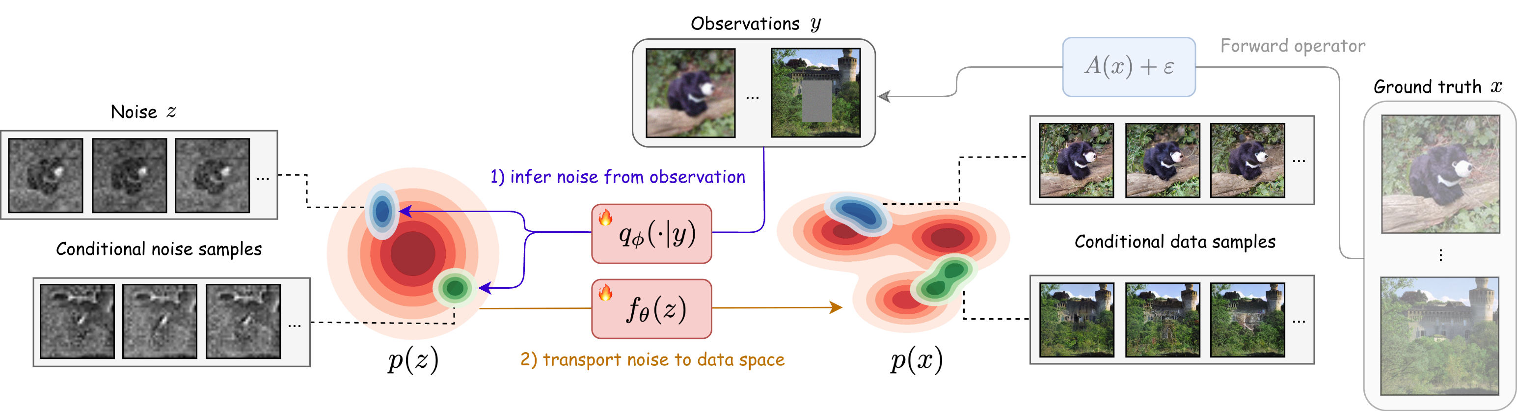
Think of a one‑step generator as a machine that turns random noise into a realistic image in one go. That’s super fast, but there’s a catch: when you want the output to match some observation (like a masked or blurry image), you can’t nudge it step by step—there is no path to steer.
The authors’ idea: instead of steering the path, pick the right starting noise.
- Noise adapter (the “chooser”): A small network looks at your observation (say, a blurry photo) and outputs a distribution of noise vectors that are likely to produce images matching that observation when passed through the generator.
- One‑step flow map (the “machine”): A model that maps a noise vector directly to a clean image in a single move.
They train both together using a variational objective (you can think of it like a VAE idea adapted to this setting):
- Observation fit: Images produced from the chosen noise should agree with what you observed (e.g., when blurred, they look like the input).
- Data fit: The result should stay on the “real image” manifold—i.e., look like real images, not artifacts.
- Regularization (keep noise sensible): The chosen noise shouldn’t be wild; it stays close to standard random noise (so the model remains stable and generalizes).
They also use a “mean flow” training rule that keeps the one‑step generator faithful to the math of continuous flows (this helps it remain high‑quality and usable in one or a few steps).
Two practical add‑ons:
- Multi‑task conditioning: The noise adapter can be told which kind of problem it’s solving (e.g., inpainting vs. deblurring), so one model can handle many tasks.
- Few‑step option: Although one step already works well, you can optionally use a handful of steps for even better quality, still much faster than hundreds.
Analogy: Imagine a vending machine that can make a full meal from a secret code (noise). If you want a vegetarian pizza, you can’t tweak the cooking midway. Instead, you learn to dial the best code from the start so the machine produces the pizza you want in one go.
What did they find and why is it important?
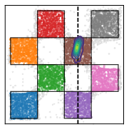
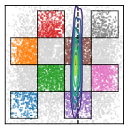
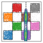
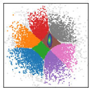
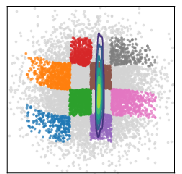
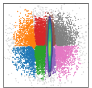
- Toy 2D test: On a simple “checkerboard” example, their method captured multiple valid answers (multimodality) better than baselines. Training the noise chooser and the generator together worked much better than training them separately.
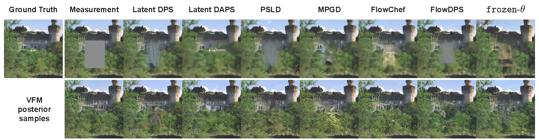
- ImageNet inverse problems (inpainting and deblurring):
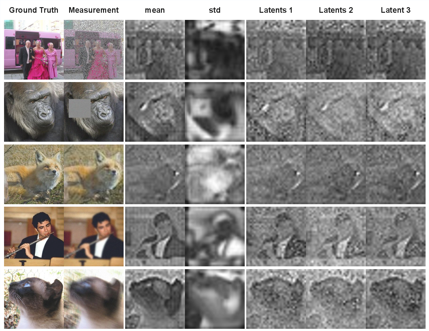
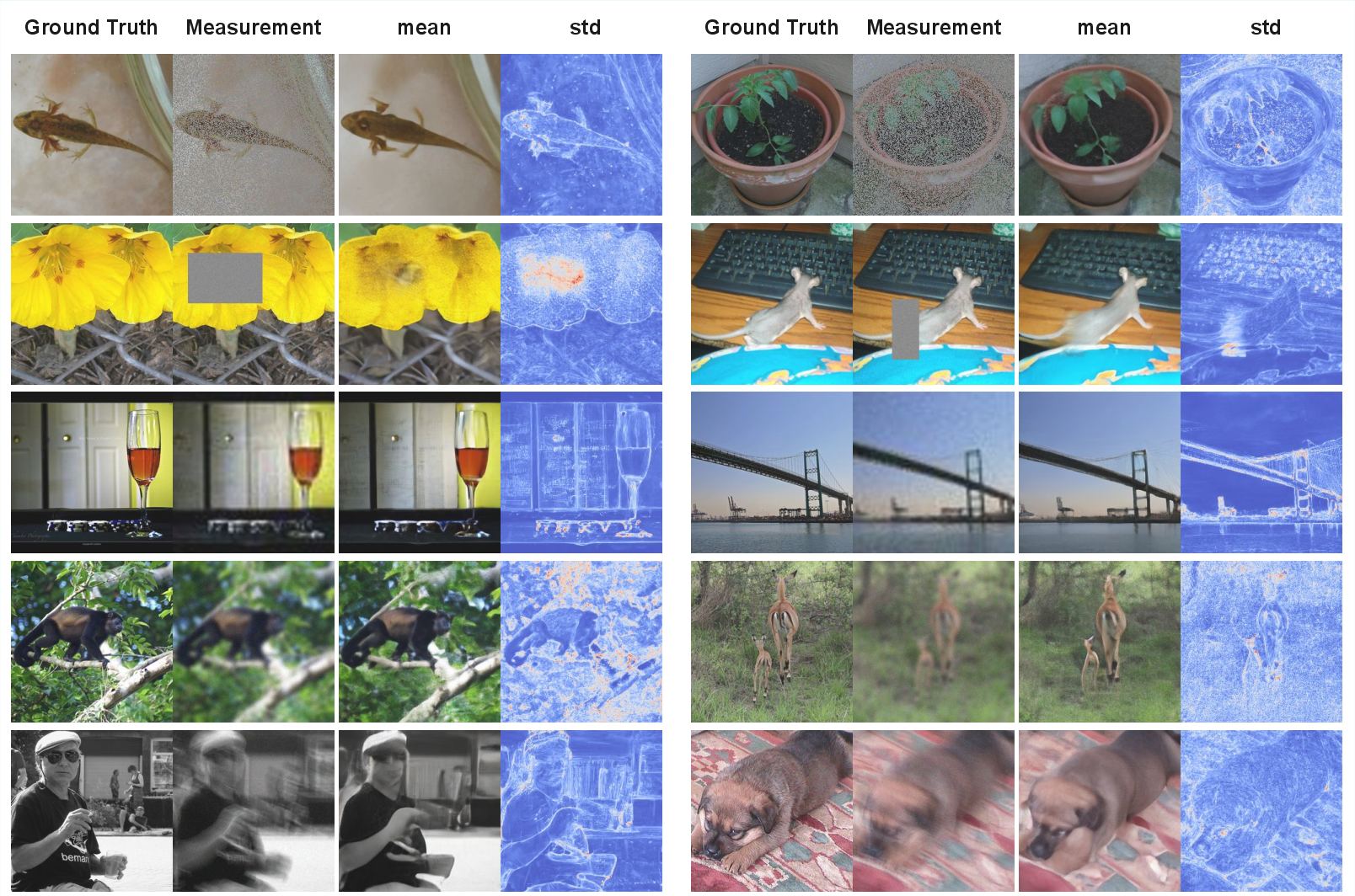
- Quality: Their one‑step (or few‑step) method produced diverse, sharp, and well‑calibrated results. It strongly improved perceptual and distributional metrics (like FID, LPIPS, MMD, CRPS), meaning outputs were both realistic and captured uncertainty well.
- Speed: It was orders of magnitude faster at inference (about hundredfold faster) than guidance‑based diffusion/flow solvers that need 250+ steps.
- Pixel scores: Traditional pixel‑by‑pixel metrics (PSNR/SSIM) sometimes favored slower iterative methods for a single sample, because those metrics prefer smoother averages. But if you average a few one‑step samples, VFM narrows or even beats the gap.
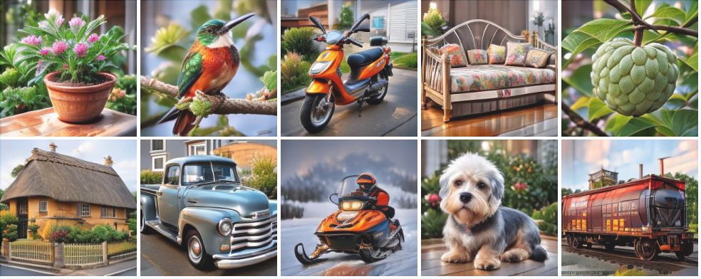
- Unconditional generation is still strong: Even after training for conditional tasks, the one‑step generator remained competitive at making diverse, high‑quality images from pure noise.
- Reward alignment (extra experiment): They showed you can fine‑tune the same framework to aim for arbitrary, differentiable “rewards” (for example, making images that better match a score or a prompt) and still generate in one step. This avoids slow, iterative fine‑tuning.
Why it matters:
- Real‑time and interactive use: One‑step or few‑step conditional generation is fast enough for apps like photo editors, AR/VR, and on‑device tools.
- Versatility: One noise adapter can handle many kinds of inverse problems by conditioning on the task.
- Better uncertainty: Producing multiple plausible answers quickly helps in science, medicine, and any setting where you want a distribution of possible reconstructions, not just one guess.
What’s the bigger picture?
This work changes how we think about conditional generation for one‑step models. Instead of guiding a long process, VFM learns to pick the right starting noise so the one‑step generator lands on good solutions immediately. That makes conditional generation far faster while staying accurate and diverse. It also opens the door to quick fine‑tuning for new goals (rewards) without heavy computation. In short, VFM brings the speed of one‑step models to many practical tasks that used to require slow, iterative methods.
Knowledge Gaps
Knowledge gaps, limitations, and open questions
Below is a concise, actionable list of what remains missing, uncertain, or unexplored in the paper that future work could address:
- Theory beyond linear-Gaussian toy settings
- Extend Proposition 1 (posterior mean recovery) to non-linear generative maps, non-Gaussian priors/likelihoods, and high-dimensional regimes.
- Provide convergence guarantees or sufficient conditions for joint optimization of (θ, φ) to approximate (e.g., bounds on the pushforward approximation error).
- Analyze identifiability and expressivity limits when is not invertible and is restricted (e.g., when many z map to the same x).
- Tightness and faithfulness of the training objective
- Quantify how tightly the mean-flow loss upper-bounds the data reconstruction term (Proposition 2) and how this relationship changes when sampling beyond the anchored case.
- Establish a principled link between the mixed objective in Eq. (12) and an ELBO-like bound on ; characterize approximation gaps introduced by substituting with a mean-flow proxy and by using stop-gradient/EMA heuristics.
- Role of τ and its inconsistency with the theoretical limit
- Theoretically, posterior sampling correctness requires (Proposition 3), but empirically training is only stable when . Develop an annealing or adaptive scheme (or an alternative objective) that preserves stability while moving toward the theoretically correct regime.
- Provide criteria or estimators to set/learn jointly with (θ, φ), and study sensitivity to τ under different noise levels and forward operators.
- Choosing and adapting α (unconditional/conditional mixing)
- Formalize how α trades off posterior fit and unconditional fidelity; derive an adaptive strategy to choose α during training (e.g., via multi-objective optimization or validation criteria).
- Analyze how α interacts with model capacity and task difficulty to prevent degradation of unconditional generation.
- Expressivity limits of the Gaussian adapter
- Quantify when a diagonal-Gaussian is provably insufficient to capture multi-modal or heavy-tailed , even with joint warping by .
- Evaluate richer adapter families (mixtures, normalizing flows, diffusion-on-latents) and measure gains vs. training cost and stability.
- Exploiting y during multi-step refinement
- Current multi-step sampling conditions only the initial noise z; subsequent steps ignore y. Investigate y-aware refinement steps (e.g., conditioning or adding observation-informed correctors) and characterize when they improve posterior accuracy.
- Robustness to model and operator mis-specification
- Study sensitivity when the forward operator A is mismatched, non-linear, unknown (blind inverse problems), or when the noise model is non-Gaussian/heteroscedastic or σ is mis-specified/unknown.
- Evaluate amortization generalization: how well does a model trained over a class of operators extrapolate to unseen operators, distributions over A, or out-of-distribution y?
- Posterior-quality evaluation at scale
- Move beyond perceptual metrics (FID/LPIPS) to posterior diagnostics on high-dimensional datasets: measurement-consistency distributions, coverage of credible sets, calibration error, conditional MMDs, or surrogate likelihood/proxy NLPD to detect under/over-dispersion.
- Quantify diversity-accuracy trade-offs and mode coverage within the conditional posterior, not just unconditional samples.
- Speed–quality Pareto and baseline fairness
- Provide thorough NFE–quality trade-off curves for guidance baselines (including tuned step counts) and for VFM multi-step sampling; report compute and wall-clock during training as well as inference.
- Compare against alternative one/few-step conditional methods (e.g., consistency-based conditioners) using identical backbones and training budgets.
- Scalability and domain breadth
- Demonstrate scaling to higher resolutions (e.g., 512–1024px), video/audio domains, and 3D data; report memory/compute footprints and stability issues.
- Assess performance on harder ill-posed problems (e.g., extreme super-resolution, compressive sensing with m ≪ d) and quantify degradation modes.
- EMA and stop-gradient design choices
- Analyze the bias introduced by evaluating with an EMA of θ and by stop-gradient operations in the loss reweighting. Determine when these heuristics help/hurt and propose principled alternatives (e.g., two-time-scale updates, proximal objectives).
- Learning or inferring σ (noise level)
- Extend VFM to handle unknown σ by jointly estimating it or conditioning on σ; study robustness to σ mis-specification and potential hierarchical Bayesian treatments.
- Generalization and stability of reward alignment
- Provide quantitative reward alignment results (e.g., CLIP/BLIP scores vs. FID/precision–recall) and analyze stability, sample efficiency, and mode collapse risks under different λ (and its relation to β in the target ).
- Introduce explicit constraints that keep samples close to the data distribution during reward fine-tuning (e.g., KL-to-prior on x, DPO-style objectives), and evaluate robustness to reward hacking or non-differentiable rewards.
- Transferability and modularity
- Test whether a VFM fine-tuned for one task (inverse problem/reward) retains performance on others; study catastrophic interference and mechanisms for preserving multi-task capabilities (e.g., adapter routing, conditional LoRA).
- Architectural and methodological generality
- Empirically validate that the framework transfers to other one-step operators (e.g., consistency models) beyond mean flows; compare how objective substitutions affect posterior quality and stability.
- Invertibility and latent–data geometry
- Characterize how the geometry induced by affects the complexity of and when joint warping can “Gaussianize” the noise posterior; develop diagnostics to detect when the induced coupling is insufficient.
- Uncertainty quantification for downstream decisions
- Evaluate whether single/few-step VFM posteriors are well-calibrated for decision-making tasks (e.g., risk-sensitive restoration), and compare against iterative samplers under identical computational budgets.
- Data efficiency and overfitting
- Study how dataset size and diversity affect adapter overfitting to training operators/conditions; investigate regularizers or data augmentation that improve generalization without degrading unconditional generation.
- Practical guidance for hyperparameters
- Provide principled procedures (or learned schedules) for τ, α, λ (reward strength), and adaptive loss constants (γ, p), including sensitivity analyses and default settings that transfer across datasets and tasks.
Practical Applications
Immediate Applications
The following applications can be deployed with current models and data, leveraging VFM’s one/few-step conditional generation, amortized adapters, and reward fine-tuning.
- One-step image inpainting, deblurring, and denoising in consumer and creative tools (Industry, Daily life; sector: software/media)
- Use case: Fill masked regions (box inpainting), restore blurred or noisy images with diverse, high-quality candidates in a single forward pass.
- Tools/workflows:
- A plug-in for image editors (e.g., Photoshop, Figma) or mobile camera pipelines that accepts a mask or blur kernel and produces one-step reconstructions; batch mode can draw multiple posterior-consistent samples for choice/averaging.
- Integration into latent diffusion pipelines (e.g., SD-VAE) using a VFM adapter head conditioned on task type.
- Dependencies/assumptions:
- Known or parameterized forward operator A (mask, kernel) and approximate noise level σ during training; adapter class label c for task routing.
- Pretrained flow map backbone (e.g., SiT-B/2) and stable τ, α hyperparameters; latent autoencoder quality limits final image fidelity.
- Real-time content-aware fill on edge devices (Industry, Daily life; sector: mobile/edge AI)
- Use case: One-step, on-device completion/cleanup of images (e.g., panoramas, social media posts), exploiting orders-of-magnitude lower NFE vs diffusion guidance.
- Tools/workflows:
- Edge inference module exposing a simple API: provide (y, c) and receive x in 1–2 NFEs.
- Mixed-precision or quantized deployment of the flow map and adapter.
- Dependencies/assumptions:
- Memory- and compute-constrained deployment; models sized appropriately.
- Domain shift control (mobile photos vs training set) to preserve calibration.
- Multi-task inverse problem solver for imagery (Industry, Academia; sector: vision/graphics)
- Use case: A single VFM model amortized over families of operators (e.g., denoising, inpainting with random masks, deblurring with kernel distributions) to deliver unified conditional generation with uncertainty estimates.
- Tools/workflows:
- “VFM-Inverse SDK” exposing adapter conditioning on class c, with operator families A_cω and optional multi-step refinement (K ≪ diffusion steps).
- Batch posterior sampling for ensembles and averaging (improves PSNR/SSIM without heavy sampling).
- Dependencies/assumptions:
- Accurate task labels and representative operator distributions during training.
- Gaussian adapter (diagonal) is assumed; joint training mitigates but does not remove expressivity limits.
- Fast posterior sampling for imaging UQ and decision support (Academia, Industry; sector: healthcare R&D, scientific imaging)
- Use case: Generate diverse, observation-consistent reconstructions and predictive intervals in seconds for prototyping (e.g., microscopy, preclinical imaging, materials).
- Tools/workflows:
- VFM posterior sampling to compute pixel-, feature-, or embedding-based uncertainty (e.g., CRPS via DINO/Inc features).
- Plug-in for lab pipelines where A is known (e.g., known point spread function).
- Dependencies/assumptions:
- Requires differentiable A during training; calibration depends on match between lab conditions and training assumptions (σ, operator family).
- Reward-aligned image generation without iterative guidance (Industry, Academia; sector: generative AI/safety)
- Use case: One-step generation biased toward differentiable rewards (e.g., aesthetic score, brand/style classifier, content safety), while staying close to data prior.
- Tools/workflows:
- “VFM-Reward FT” fine-tunes adapter and flow map with a reward loss in <0.5 epochs and deploys a 1-NFE sampler; can be used to enforce house style or safety filters in content platforms.
- Dependencies/assumptions:
- Rewards must be differentiable and well-calibrated; choose λ to balance quality/diversity vs reward hacking.
- Guardrails may still be needed (post-hoc filters, classifier-free checks).
- Remote sensing quick fixes: deblurring, inpainting, cloud-gap filling (Industry, Academia; sector: geospatial)
- Use case: Fast posterior-consistent fills of cloud-covered or blurred satellite patches for rapid triage and analyst workflows.
- Tools/workflows:
- VFM service where c indexes operator families (cloud masks, kernels) and outputs multiple consistent fills for analyst selection.
- Dependencies/assumptions:
- Training data must reflect sensor properties; performance tied to autoencoder latent quality and A realism.
- Dataset augmentation with constraint-consistent variants (Industry, Academia; sector: ML engineering)
- Use case: Generate multiple plausible labeled variants consistent with synthetic degradations (supervision for robustness).
- Tools/workflows:
- Automatic pipeline applying A_cω to x, sampling VFM posterior, and attaching provenance; useful for training restoration or detection models.
- Dependencies/assumptions:
- Careful curation to avoid bias; adherence to licensing and data provenance policies.
- Energy/carbon efficiency in generative inference (Policy, Industry; cross-sector)
- Use case: Replace 250-step guidance pipelines with 1–2 step VFM samplers to cut inference energy demand in deployment.
- Tools/workflows:
- Internal reporting and sustainability dashboards tracking NFE and wall-clock per request; adoption in green-ops initiatives.
- Dependencies/assumptions:
- Equivalent or better task quality must be verified for policy targets; model updates may shift compute/energy back to training rather than inference.
Long-Term Applications
These applications are feasible with further research, domain adaptation, and validation (e.g., robust operators A, non-image modalities, regulatory processes).
- Clinical imaging reconstruction with calibrated uncertainty (Industry, Policy, Academia; sector: healthcare/medical imaging)
- Use case: One/few-step reconstruction from undersampled MRI, low-dose CT, PET with posterior samples for radiologist confidence.
- Tools/products:
- VFM-based recon software integrated with scanner pipelines; fast posterior ensembles for UQ overlays.
- Dependencies/assumptions:
- High-fidelity, regulated, modality-specific A (sensor physics), thorough validation, bias/fairness audits; medical-device compliance (e.g., FDA/CE).
- Scientific and industrial PDE-constrained inverse problems (Academia, Industry; sector: energy, materials, climate)
- Use case: Rapid posterior sampling for seismic imaging, non-destructive testing, tomography, or climate data assimilation where A encodes complex physics.
- Tools/workflows:
- Hybrid VFM with physics-informed differentiable simulators for A; operator-class amortization over parameterized PDEs.
- Dependencies/assumptions:
- Efficient, differentiable physics solvers; scalable training; managing mismatch between simulator and real-world data; adapter expressivity may need upgrading beyond diagonal Gaussian.
- Real-time AR/VR occlusion reasoning and scene completion with UQ (Industry; sector: XR/robotics)
- Use case: Single-pass completion of occluded views or depth/color gaps with confidence maps to reduce visual artifacts in headsets.
- Tools/workflows:
- On-headset VFM components with low-latency budget; optional multi-step K=2–4 refinement for hard cases.
- Dependencies/assumptions:
- Tight latency and memory constraints; robust handling of motion/temporal consistency; domain-specific operators (e.g., sparse depth A).
- Reward-aligned safety and policy enforcement at generation time (Policy, Industry; sector: online platforms)
- Use case: Single-step alignment to safety rewards (nudity/violence/brand safety), stylistic compliance, and watermark adherence at scale.
- Tools/workflows:
- Platform-level VFM fine-tuning to policy-defined rewards; dynamic reweighting λ to adapt to new policies; continuous evaluation.
- Dependencies/assumptions:
- Reliable, unbiased differentiable safety surrogates; governance for reward hacking and failure cases; audit trails for compliance.
- Time-series and multimodal conditional generation (Industry, Academia; sector: finance, speech/audio, video)
- Use case: Conditional scenario generation (e.g., market stress tests given observed factors), audio/video inpainting or denoising with posterior diversity in few steps.
- Tools/workflows:
- VFM extensions with sequence-aware flow maps and adapters; task-specific A (e.g., downsampling/masking in time).
- Dependencies/assumptions:
- Non-image latent spaces and encoders; stable training for sequential flow maps; domain-specific evaluation and risk controls (especially in finance).
- Privacy-preserving imputation and synthetic data with constraints (Policy, Industry, Academia; sector: data governance)
- Use case: Fast, constraint-consistent imputation or synthetic sample generation under privacy budgets; reproducible posterior draws.
- Tools/workflows:
- Differentially private training of VFM; adapters conditioned on observed subsets/masks; publishing uncertainty bounds.
- Dependencies/assumptions:
- DP mechanisms integrated into training; careful calibration and privacy accounting; legal/ethical compliance.
- Automated design space exploration with constraints (Industry, Academia; sector: manufacturing, materials, bio)
- Use case: Generate multiple candidate designs consistent with measurements or constraints (e.g., target spectra, shapes) for downstream screening.
- Tools/workflows:
- VFM conditioned on measured properties via A, producing posterior-consistent design candidates in one step; plug into optimization loops.
- Dependencies/assumptions:
- Differentiable, faithful A mapping designs to observables; domain-specific priors; extensions beyond images to meshes, molecules, or CAD.
- Remote sensing at scale with physics-aware operators (Industry, Academia; sector: geospatial)
- Use case: Planet-scale inpainting/deblurring with per-pixel UQ, integrating orbit/sensor physics in A to improve fidelity.
- Tools/workflows:
- VFM with learned or hybrid physics operators; multi-sensor conditioning; active learning for hard regions.
- Dependencies/assumptions:
- High-quality, multi-sensor datasets; handling of heavy-tailed noise and non-Gaussian effects; scalable distributed inference.
- On-device generative co-pilots with energy-aware inference (Industry, Policy; sector: consumer devices)
- Use case: Assistant features (background edits, content-aware actions) that meet energy budgets and privacy constraints by avoiding iterative guidance.
- Tools/workflows:
- Co-processor or NPU-optimized VFM implementation; user-controlled UQ for transparency (e.g., show diversity/confidence).
- Dependencies/assumptions:
- Hardware-software co-design; product UX for uncertainty; continual learning to adapt to user domains.
Cross-cutting assumptions and dependencies (affecting feasibility)
- Forward operator A must be known/learnable and ideally differentiable during training; mismatches degrade calibration.
- Gaussian, diagonal-covariance adapter is a simplifying assumption; joint training helps but may be insufficient for highly multi-modal posteriors without richer adapters.
- Hyperparameters τ (data coupling) and α (unconditional mixing) are critical for stability/performance; τ ≫ σ often stabilizes training but changes the exactness of posterior matching.
- Operating in latent space ties performance to the quality of the autoencoder/decoder.
- Reward-aligned fine-tuning requires reliable, differentiable reward functions and safeguards against reward hacking; λ must balance fidelity and alignment.
- Domain shifts (data, operators, noise) require retraining or robust amortization; multi-task generalization depends on representative training coverage.
Glossary
- Adaptive loss: A stabilization technique that rescales the training objective dynamically to prevent optimization instabilities. "we consider an adaptive loss scaling to stabilize optimization."
- Amortized variational inference: Using a neural network to map conditioning variables directly to parameters of a variational posterior, enabling fast approximate inference across many instances. "approximates the noise space posterior via amortized variational inference."
- Average velocity: An integrated characterization of flow dynamics over a time interval that enables direct one-step transport in flow maps. "which introduce the average velocity as an alternative characterization:"
- Bayesian inverse problem: Recovering an unknown signal from noisy observations by combining a likelihood model with a prior to form a posterior distribution. "Formulating this as a Bayesian inverse problem, we can derive a principled variational training objective"
- Classifier-free guidance: A sampling technique that steers generative models toward a condition without an explicit classifier, often incurring extra compute. "with an additional × 2 cost for classifier-free guidance"
- Consistency models: Generative models that learn mappings consistent along a diffusion or flow trajectory, enabling few-step sampling. "Consistency models~\citep{song_consistency_2023}, for example, learn to map any point on the flow trajectory directly to the corresponding clean data"
- Continuous Ranked Probability Score (CRPS): A proper scoring rule measuring calibration and sharpness of probabilistic predictions against observed outcomes. "the continuous ranked probability score (CRPS) measures uncertainty calibration around the ground truth that generated "
- Conjugate variational posterior: A variational family chosen to be conjugate to the prior/likelihood for tractable divergence terms and efficient optimization. "imposing a conjugate variational posterior, such as "
- Evidence Lower Bound (ELBO): A variational objective that lower-bounds the log-evidence and is maximized to fit generative models and inference networks. "is the negative evidence lower bound (ELBO)"
- Exponential Moving Average (EMA): A smoothing technique over model parameters used to stabilize training and evaluation. "with its exponential moving average (EMA)"
- Eulerian condition: A structural property of ODE flows used to constrain and train flow-map parameterizations. "trained on the so-called Eulerian condition satisfied by ODE flows."
- Flow map: A learned operator that maps noise directly to data (and between times) in one or few steps, emulating the solution of an ODE-driven generative process. "Flow maps enable high-quality image generation in a single forward pass."
- Flow matching: A training objective that regresses model velocities to target velocities along interpolants between data and noise to learn generative flows. "Flow matching~\citep{lipman2022flow, liu2022flow, albergo2023stochastic} provides a training objective to learn "
- Forward operator: The known transformation from latent signals to observations in an inverse problem. "is a known forward operator"
- Fréchet Inception Distance (FID): A feature-space metric comparing distributions of real and generated images via Gaussian approximations in Inception features. "we achieve an FID of 33.3."
- Guidance-based methods: Iterative sampling approaches that incorporate likelihood or condition gradients to steer generative trajectories toward conditional targets. "guidance-based methods~\citep{chung2024diffusionposteriorsamplinggeneral, song2023pseudoinverseguided} approximate posterior sampling"
- Inverse problem: Estimating an unknown signal from indirect or noisy measurements, typically under a forward model and noise. "Inverse problem seeks to recover an unknown signal from noisy observations"
- Kullback–Leibler divergence (KL): A measure of discrepancy between two probability distributions, used as the optimization objective in variational inference. "Kullback-Leibler (KL) divergence:"
- Latent space: A lower-dimensional representation space in which generative models operate or sample, often with a simple prior. "All methods operate in the latent space of SD-VAE \cite{rombach2022high}."
- Learned Perceptual Image Patch Similarity (LPIPS): A perceptual similarity metric based on deep features, correlating better with human judgment than pixel metrics. "On LPIPS, which is a feature-space perceptual similarity metric, we find that VFM is competitive"
- Linear interpolant: A straight-line path between data and noise used to define training targets for flow/diffusion models. "we construct a linear interpolant "
- Maximum Mean Discrepancy (MMD): A kernel-based distance between distributions measured via differences in feature means. "the maximum mean discrepancy (MMD) provides a sample-based distance between the true and approximate posteriors"
- Mean flow: A flow-map parameterization based on average velocities enabling one-step generation with structural guarantees. "the state-of-the-art Mean Flow model \cite{geng2025meanflowsonestepgenerative}"
- Mean flow loss: The regression loss that enforces consistency of the learned average velocity with the implied ODE structure across times. "the mean flow loss is given by"
- Ordinary Differential Equation (ODE): A continuous-time dynamical system describing the evolution of samples between noise and data distributions. "based on ordinary or stochastic differential equations (ODE/SDEs)"
- Peak Signal-to-Noise Ratio (PSNR): A pixel-space fidelity metric measuring reconstruction error relative to signal range. "On pixel-space fidelity metrics (PSNR, SSIM), guidance methods consistently scores higher than a single VFM draw."
- Pushforward (measure): The distribution obtained by transforming a random variable through a deterministic function. "converges weakly to the pushforward of the noise-space posterior under the map "
- Reward alignment: Fine-tuning a generative model so that its samples maximize a differentiable reward while staying close to the data distribution. "a highly efficient framework for general reward alignment."
- Reward-tilted distribution: A distribution reweighted by an exponentiated reward function to favor high-reward samples. "sampling from a reward-tilted distribution $p_{\text{reward}(x|c) \propto p_{\text{data}(x) \exp(\beta R(x, c))$."
- Semi-group property: A compositional property of flows stating that evolution over time intervals composes consistently, important for flow-map structure. "such as the semi-group property \citep{boffi2025build}"
- Stochastic Differential Equation (SDE): A dynamical system with stochastic noise used to define generative processes between distributions. "based on ordinary or stochastic differential equations (ODE/SDEs)"
- Support Accuracy (SACC): The proportion of generated samples that lie within the valid support/manifold of the target distribution. "the support accuracy (SACC) measures the proportion of samples that lie on the checkerboard support."
- Two-time flow map: A flow-map operator that maps a state at time t to another time s, enabling flexible step counts at inference. "the two-time flow map learns to approximate "
- Variational Autoencoder (VAE): A generative model that jointly trains an encoder and decoder via the ELBO to approximate posteriors and data likelihoods. "A prototypical example is the {\em Variational Autoencoder (VAE)}"
- Variational Flow Maps (VFM): A framework that pairs a flow map with a noise adapter trained via a variational objective to enable one/few-step conditional generation. "Variational Flow Maps, a framework for conditional sampling"
- Variational posterior: A tractable distribution used to approximate an intractable true posterior by minimizing KL divergence. "introducing a variational posterior "
- Velocity field: The time-dependent vector field governing the dynamics of the flow between distributions. "where is a time-dependent velocity field."
- Weak convergence: Convergence in distribution of probability measures, often used to justify limiting behaviors of learned models. "converges weakly to the pushforward of the noise-space posterior under the map "
Collections
Sign up for free to add this paper to one or more collections.