Flow Matching with Semidiscrete Couplings
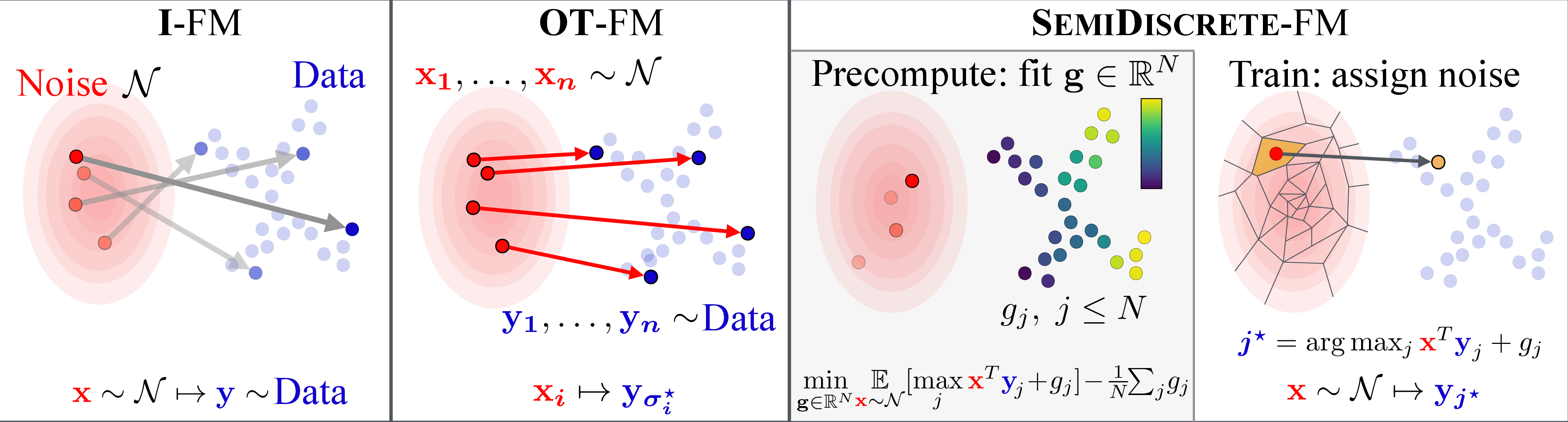
Abstract: Flow models parameterized as time-dependent velocity fields can generate data from noise by integrating an ODE. These models are often trained using flow matching, i.e. by sampling random pairs of noise and target points $(\mathbf{x}_0,\mathbf{x}_1)$ and ensuring that the velocity field is aligned, on average, with $\mathbf{x}_1-\mathbf{x}_0$ when evaluated along a segment linking $\mathbf{x}_0$ to $\mathbf{x}_1$. While these pairs are sampled independently by default, they can also be selected more carefully by matching batches of $n$ noise to $n$ target points using an optimal transport (OT) solver. Although promising in theory, the OT flow matching (OT-FM) approach is not widely used in practice. Zhang et al. (2025) pointed out recently that OT-FM truly starts paying off when the batch size $n$ grows significantly, which only a multi-GPU implementation of the Sinkhorn algorithm can handle. Unfortunately, the costs of running Sinkhorn can quickly balloon, requiring $O(n2/\varepsilon2)$ operations for every $n$ pairs used to fit the velocity field, where $\varepsilon$ is a regularization parameter that should be typically small to yield better results. To fulfill the theoretical promises of OT-FM, we propose to move away from batch-OT and rely instead on a semidiscrete formulation that leverages the fact that the target dataset distribution is usually of finite size $N$. The SD-OT problem is solved by estimating a dual potential vector using SGD; using that vector, freshly sampled noise vectors at train time can then be matched with data points at the cost of a maximum inner product search (MIPS). Semidiscrete FM (SD-FM) removes the quadratic dependency on $n/\varepsilon$ that bottlenecks OT-FM. SD-FM beats both FM and OT-FM on all training metrics and inference budget constraints, across multiple datasets, on unconditional/conditional generation, or when using mean-flow models.


Paper Prompts
Sign up for free to create and run prompts on this paper using GPT-5.
Top Community Prompts
Explain it Like I'm 14
What is this paper about?
This paper is about teaching computers to turn random noise into realistic data, like images, by following smooth, easy-to-compute paths. The authors introduce a new way to pick “good pairs” between noise and real data during training so the model learns straighter, simpler paths. Their method, called Semidiscrete Flow Matching (SD-FM), keeps the benefits of an advanced math tool (optimal transport) but avoids its usual heavy compute cost.
What questions are the authors trying to answer?
- How can we pick better noise–data pairs during training so the model learns to move from noise to data along straighter, easier paths?
- Can we do this without the big, slow computations used by earlier optimal-transport-based methods?
- Can we measure and guarantee that our pairing method is actually learning the right thing?
- Will this make models faster and better across many tasks, like unconditional generation, class-conditional generation, and image super-resolution?
How does the method work?
Flow matching in one sentence
Imagine you have a “wind field” that pushes points in space. If you start with random points (noise) and push them along this wind over time, they should end up looking like real data (e.g., images). Training teaches the wind which way to blow. This is called flow matching.
Why choosing pairs matters
To teach the wind, you repeatedly show the model a pair: one noise point and one real data point. You also pick a random time between start and finish, and ask the wind to point from where you are now toward the target. If you pair noise and data randomly, the model can still learn—but the paths it learns often curve a lot, which makes generation slower and lower quality.
The old way: batch optimal transport (OT)
Optimal transport is like the world’s best delivery planner: it matches senders (noise) to receivers (data) to minimize total travel effort. Prior work used OT on small batches (e.g., match 256 noise points to 256 data points). In theory this makes straighter paths. In practice:
- Small batches give unstable matches.
- Big batches would be better, but they’re very expensive to compute (cost grows roughly with the square of the batch size and gets worse when you try to make it more precise).
The new way: semidiscrete OT (SD-OT) for flow matching (SD-FM)
The authors avoid matching batches against batches. Instead, they:
- Treat the dataset as a fixed list of N points.
- Learn a simple “score” (a vector of N numbers, one per data point) using standard SGD (a common training loop).
- During flow matching training, each fresh noise sample is matched to a data point by a quick lookup: “which data point gives the best score with this noise?” That’s essentially a fast nearest-better-match search.
Think of it like this:
- Batch OT: repeatedly solve a big, expensive group-matching puzzle.
- SD-FM: solve one small pre-problem once (learn per-item scores), then do fast one-by-one matching during training.
This keeps the matching smart (OT-like) but dramatically lowers the cost.
A note on ε (epsilon)
Epsilon controls how “soft” or “hard” the matching is:
- Large ε: pairs are more random (closer to independent pairing).
- Small ε: each noise is matched more deterministically to one best data point. The authors show their method works for both, and small ε often works best in practice—and is fast with their approach.
What did they find, and why is it important?
- Better image quality with less compute:
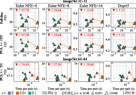
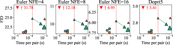
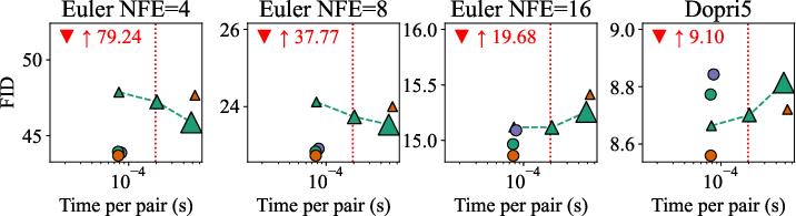
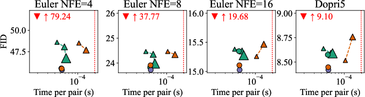
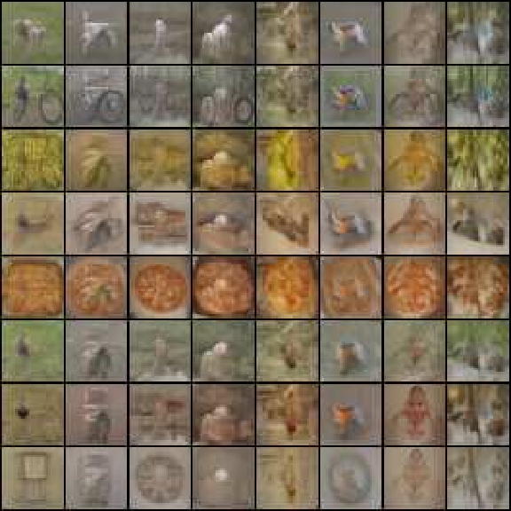
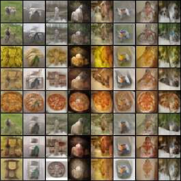
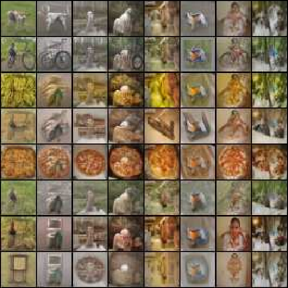
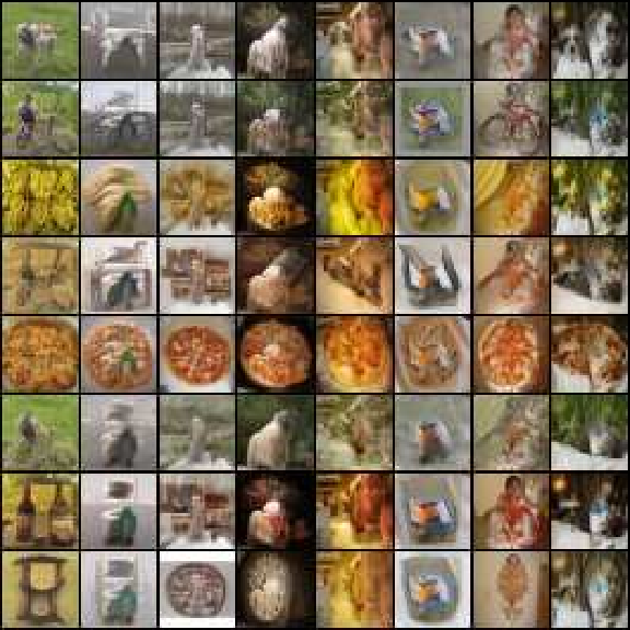
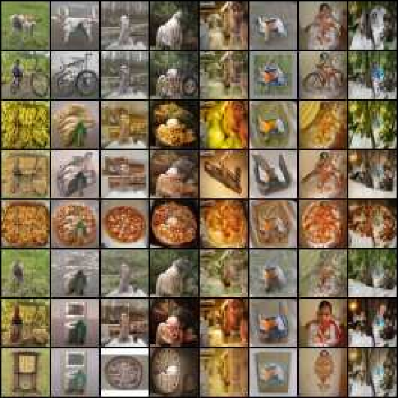
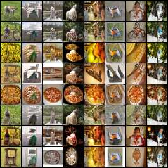
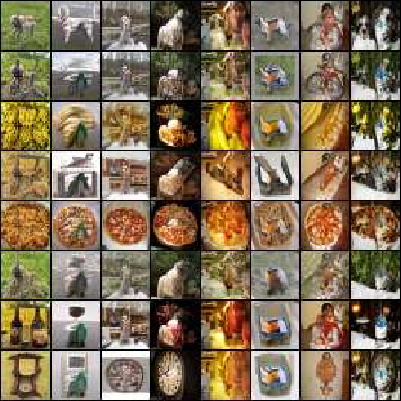
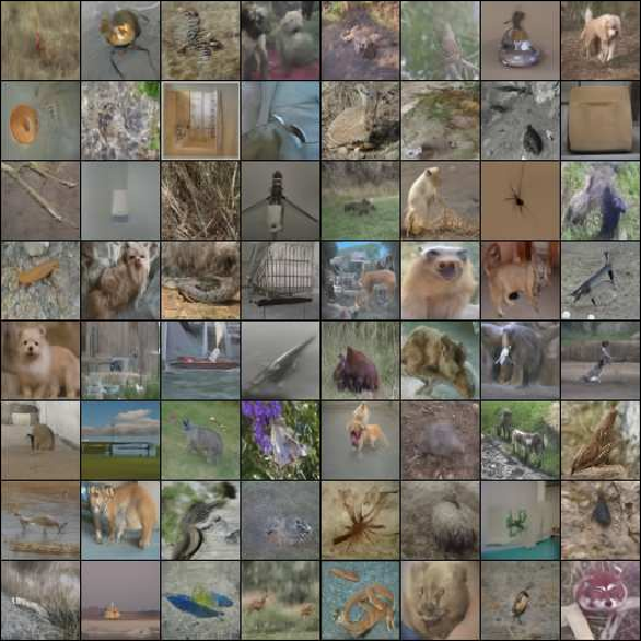
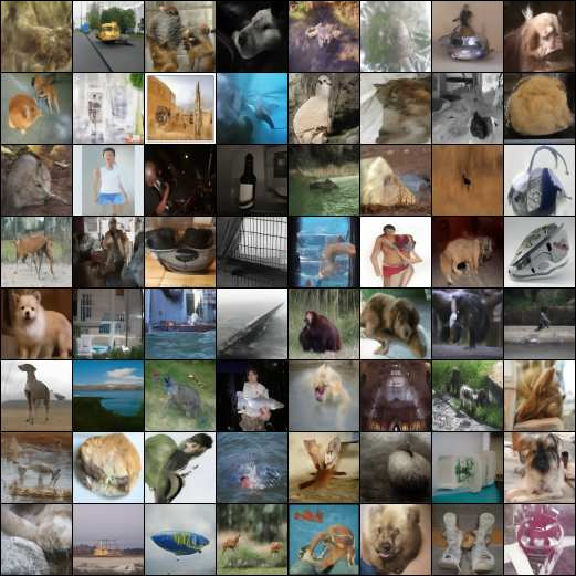
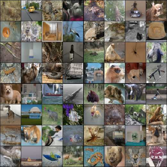
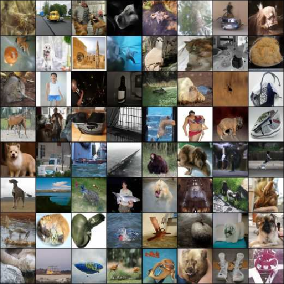
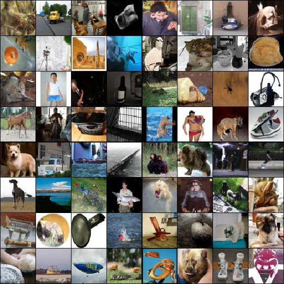
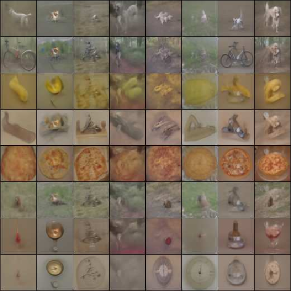
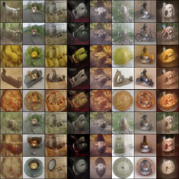
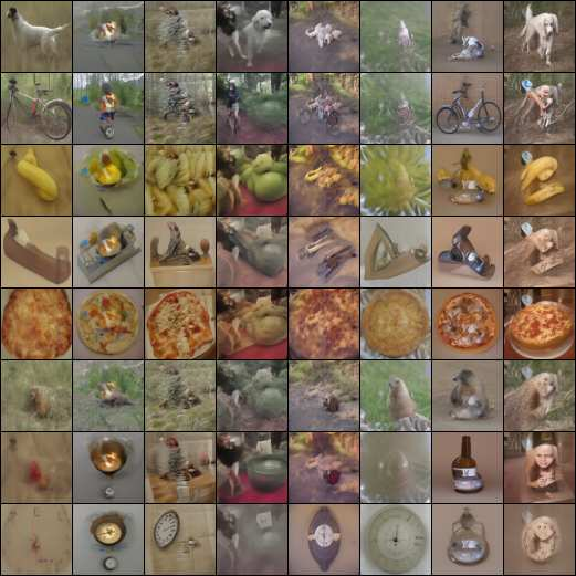
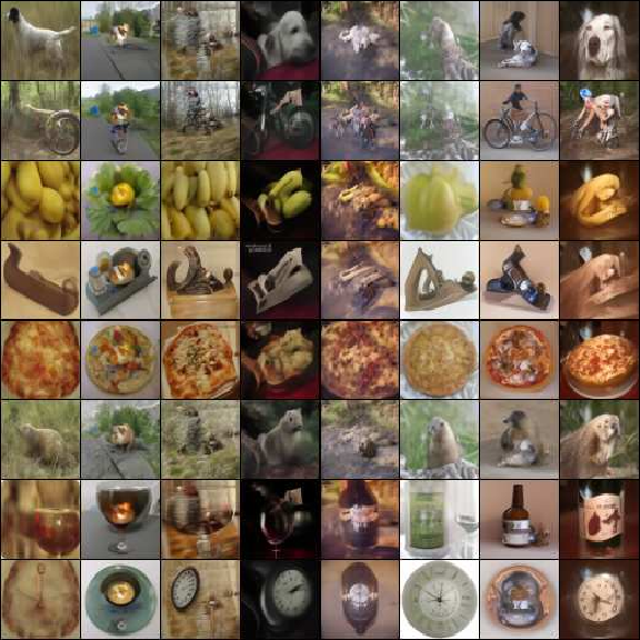
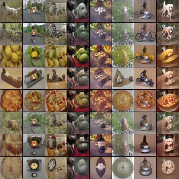
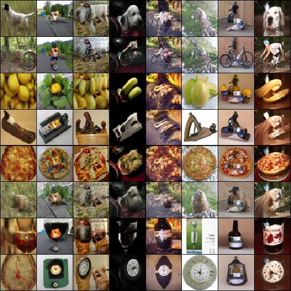
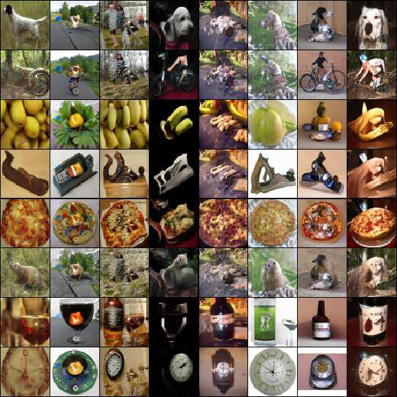
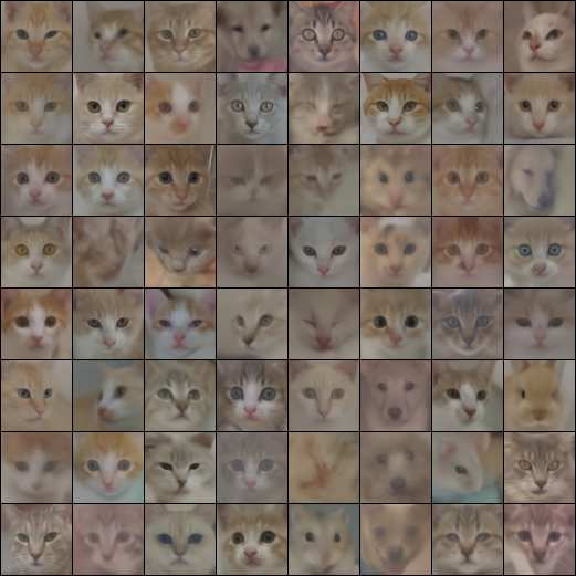
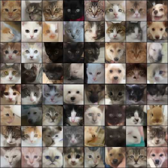
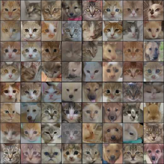
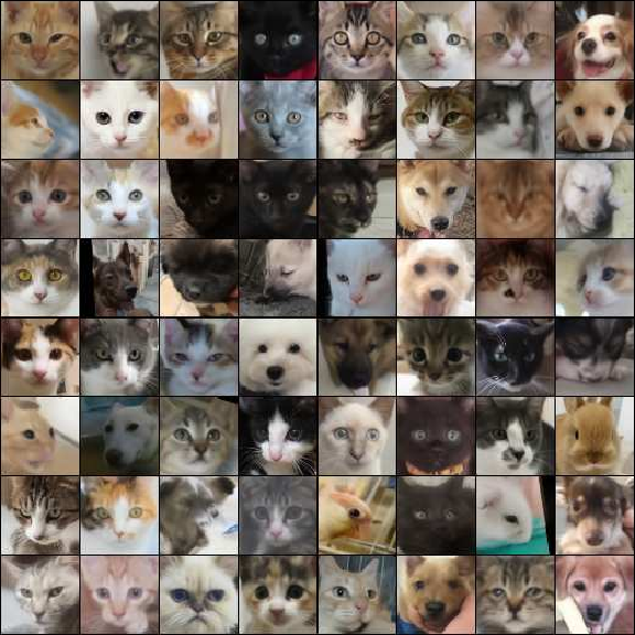
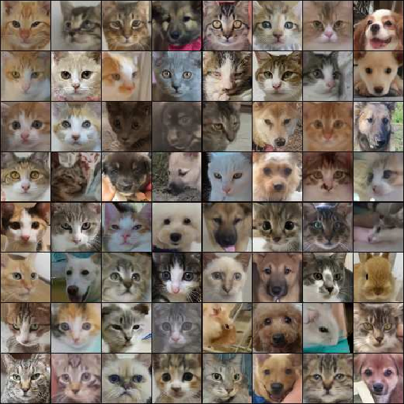
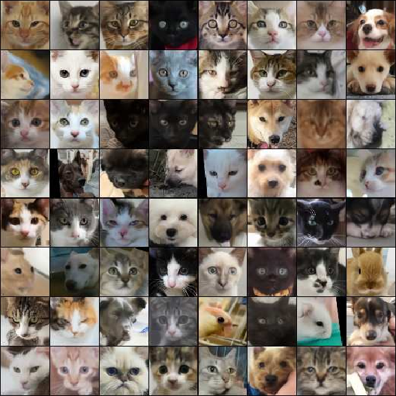
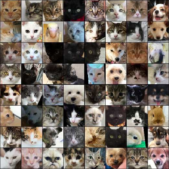
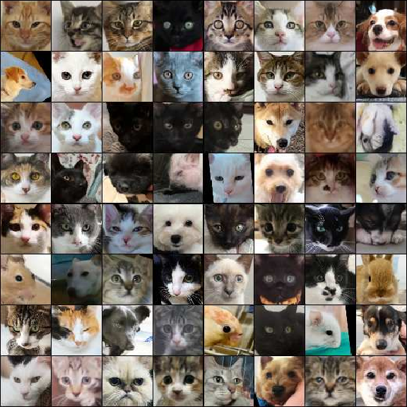
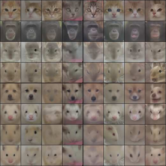
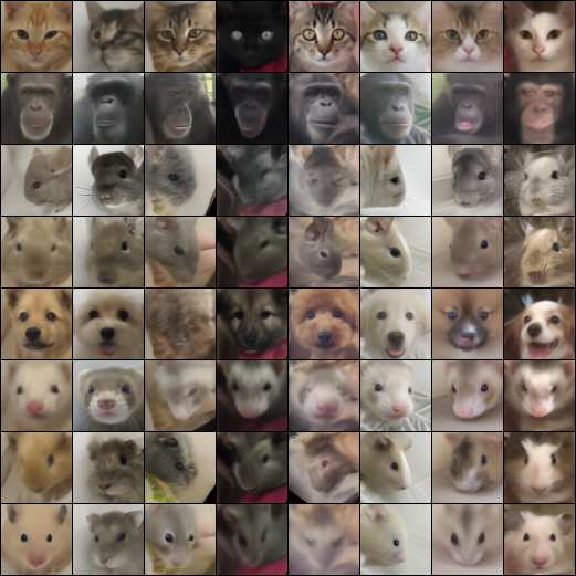
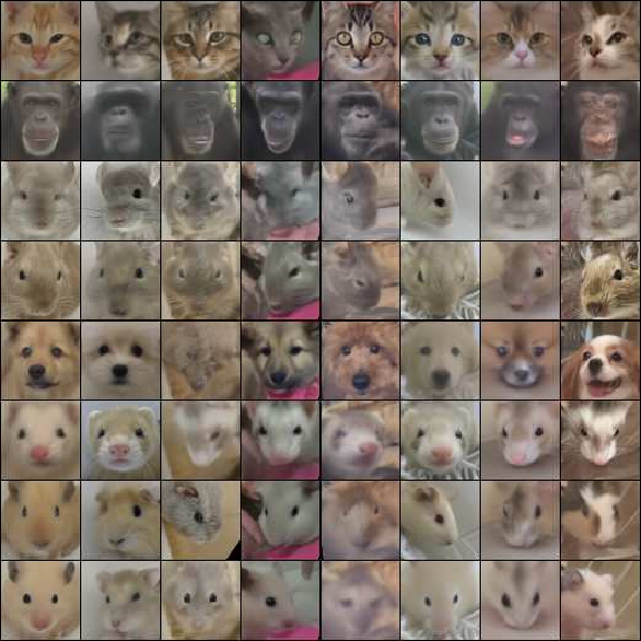
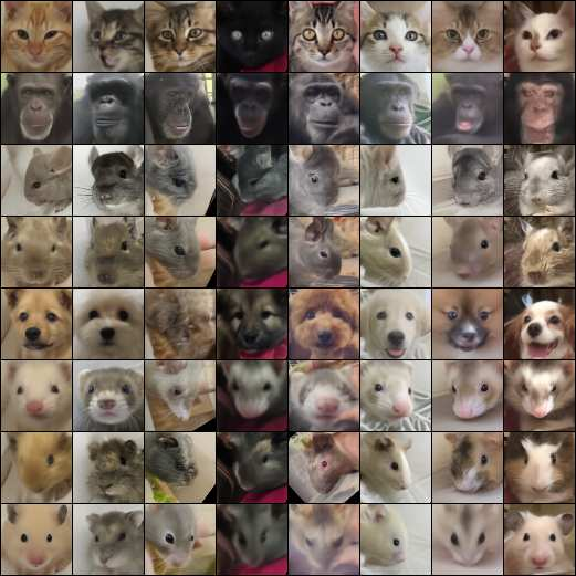
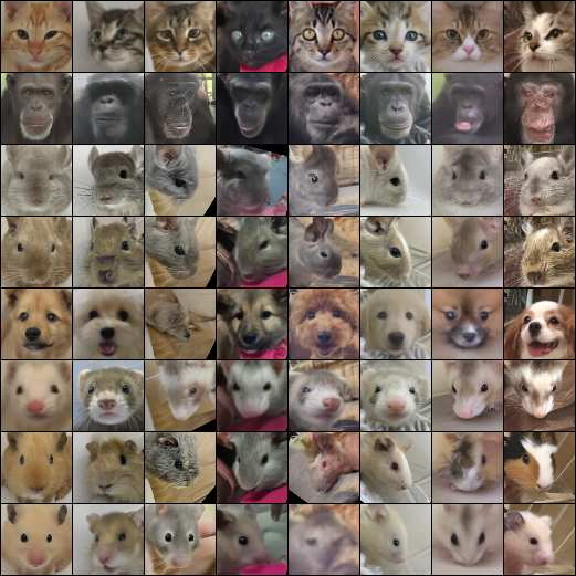
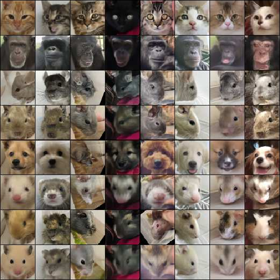
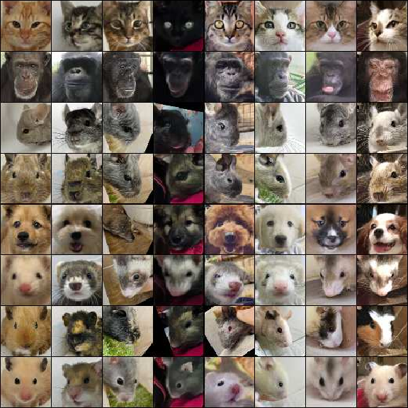
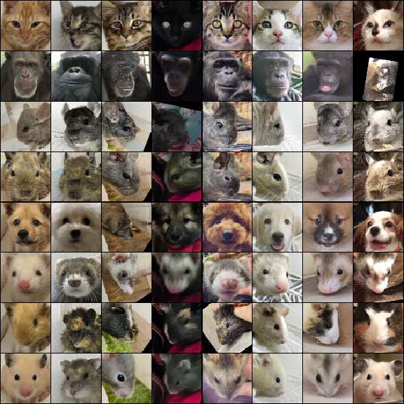
- On multiple datasets (ImageNet at 32×32 and 64×64, PetFace 64×64), SD-FM consistently beats standard flow matching (random pairing) and also beats the batch-OT approach at the same or lower pairing cost.
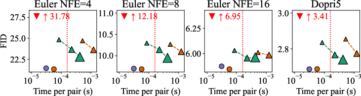
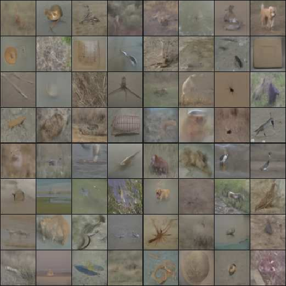
- Results are especially strong when you want to generate quickly (few ODE steps): SD-FM learns straighter paths, so it needs fewer function evaluations to make good images.
- Much cheaper pairing:
- Batch OT gets very expensive as you scale up. SD-FM avoids that by learning a single vector once, then doing fast lookups per sample.
- In practice, the extra time SD-FM needs to pick pairs is tiny compared to the normal training cost.
- Works in many settings:
- Unconditional generation (just “make a realistic image”).
- Class-conditional generation (e.g., “make a dog” or “make a car”).
- Super-resolution (turn a small, blurry image into a sharper, larger one).
- Mean-flow one-step generation settings (fast, few-step methods).
- A simple, reliable way to know training is converging:
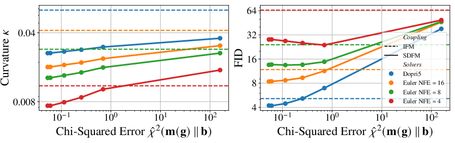
- They introduce an easy-to-compute number that tells you whether your semidiscrete pairing model has “learned enough.” It’s unbiased and efficient to estimate from samples.
- Theoretical guarantees:
- They prove that their simple SGD training for the semidiscrete pairing converges (gets close to the best possible matching) under common conditions, even when ε is zero.
- A bridge between “velocity” and “score”:
- In flow models, the “velocity field” says where to move next, while the “score” (from diffusion models) says how likely each point is. The authors show a formula that links the two for their method, with a correction that disappears when ε is very small or very large. This helps unify ideas from flows and diffusion, and supports better guidance techniques.
- Better guidance (like classifier-free guidance):
- When you blend models (for example, mixing a conditional and an unconditional model), the authors show how to correct the blend so you truly sample from the intended mixture. This can boost precision while controlling diversity.
What’s the potential impact?
- Faster, better generative models: By learning straighter, simpler paths from noise to data, SD-FM makes sampling faster and often improves quality.
- Scales to large datasets: Because it avoids the heavy cost of batch OT, SD-FM is practical for modern, large-scale training.
- Flexible and broadly useful: It works for unconditional and conditional tasks, continuous conditions (like super-resolution), and even for newer fast-generation methods.
- Strong theory and simple practice: You get a convergence meter, convergence guarantees, and a clean way to connect flow and diffusion ideas.
In short, SD-FM keeps the good parts of optimal transport without the big computational bill, leading to better training, faster inference, and strong results across tasks.
Knowledge Gaps
Knowledge gaps, limitations, and open questions
Below is a single, actionable list of gaps and open questions left unresolved by the paper.
- Convergence analysis is restricted to the neg-dot-product cost
c(x,y) = -x^T yand assumptions like minimum point separationδ > 0and bounded “surface area” ofμ; extension to other costs (e.g., squared Euclidean, augmented conditional costs), non-Gaussianμ, and realistic data duplications (i.e.,δ ≈ 0) is not provided. - The SGD rate in Theorem 1 depends on an unknown duality gap
Δ = F^*_ε − F_ε(g)to set the learning rate; practical procedures to estimate or boundΔonline (or substitute adaptive schedules with provable guarantees) are missing. - The unbiased
χ²(m(g) || b)convergence monitor is proposed, but there is no variance analysis, sample complexity bound (inBandN), or guidance for tolerances and early stopping criteria that guarantee a target accuracy on the second marginal. - The
χ²estimator and marginal computation areO(NB)per estimate; for very largeN(e.g., 109 scale), strategies for sublinear-time estimation (sketching, blockwise estimates, streaming) with error guarantees are not developed. - For
ε = 0at train time, every noise sample is assigned to a single data point via MIPS ong_j + ⟨x_0, x^{(j)}_1⟩; the effect of approximate retrieval (HNSW/FAISS, PQ/OPQ, quantization) on pairing quality, training stability, curvature, and FID is not quantified. - For
ε > 0, per-pair categorical sampling overNlogits isO(N); sublinear sampling (e.g., top-k preselection, locality-sensitive hashing, importance sampling) and the resulting bias–variance trade-offs for FM training are not explored. - MIPS indexing must incorporate additive per-point potentials
g_j; index designs that support “shifted inner products” efficiently (and their accuracy/compute trade-offs) are not described. - PCA-based pairing (using
k = 500components) changes the geometry of the cost used to computegand assignment; a systematic study of howkinfluences SD-OT accuracy and downstream FID/NFE-curvature, and guidelines for choosingk, are absent. - The role and tuning of the conditioning temperature
βinc((x,z),(x',z')) = c_x(x,x') + β c_z(z,z')are not ablated; a principled way to setβ(e.g., via calibration or validation metrics) is not provided. - Handling class/condition imbalance via non-uniform target weights
b_jis not addressed; procedures to set/learnb(and maintainm(g) = b) under imbalance or reweighting are missing. - The semidiscrete coupling is computed once and kept fixed; whether updating
gduring FM training (online/periodic refresh,ε-tempering, momentum, or batching) improves outcomes, and how to do so efficiently and stably, is unexplored. - The proposed Laguerre-cell–restricted noise sampling to improve dataloader efficiency is suggested but not implemented; algorithms to sample
X_0 ~ 𝓝(0,I)conditioned to a cellℒ_j(and their effect on pairing bias and training speed) are open. - The generalized Tweedie formula (Proposition 4) introduces a correction term
_ε; rigorous bounds on its magnitude (as a function ofε, dimension, and cost), conditions for when it is negligible, and empirical validation of score estimates are missing. - Proposition 5 (guidance corrector) is stated informally; a formal theorem with assumptions, finite-
rerror bounds, and convergence rates (plus practical discretization of the time integral and runtime profiles) is not provided. - The guidance scheme requires accurate scores; while the paper argues scores are available for
ε = 0orε = ∞, the practicality and accuracy of score estimation for smallε > 0(using the correction term), and its empirical impact on guidance, are not validated. - There is no theoretical link proving that SD-FM reduces kinetic energy or ODE curvature (least-action) compared to I-FM; only empirical evidence is shown. A bound tying SD-OT coupling quality to curvature/NFE reductions would be valuable.
- Failure modes of hard assignments at
ε = 0(e.g., many noise samples mapped to a few data points, overfitting or reduced diversity) are not analyzed; remedies (temperature smoothing, top-k stochastization, entropy floor) and their effects are not studied. - The convergence assumptions for
ε = 0requireδ > 0; real datasets often have near-duplicates, violating this assumption. Robust variants (e.g., smallε > 0, margin regularization, clustering) and their theoretical backing are missing. - Distributed training implications (multi-GPU/node): how to shard
g, perform fast global retrieval across workers, maintain consistent pairing, and avoid becoming I/O-bound whenNis large are not discussed. - Memory/computation budgets are argued to be dominated by the FM gradient
Θ, but thresholds and regimes where SD-FM pairing cost is non-negligible (small models, largeN, limited memory bandwidth) are not quantified. - Extension beyond pixel-space and latent-space flows: results are limited to ImageNet-32/64, PetFace-64, CelebA SR, and a latent-space MeanFlow at 256; scalability to high-res pixel-space (e.g., 256×256 and beyond) and other modalities (audio, text, 3D) remains to be demonstrated.
- Interaction with advanced FM-based training strategies (e.g., Reflow, consistency training variants, trajectory-regularized objectives) is left for future work; whether SD couplings complement or conflict with these methods should be empirically and theoretically assessed.
- Choice of cost function for conditions (e.g., one-hot labels with dot product) may not reflect semantic similarity; alternative condition costs (graph-based, metric-learning embeddings) and their effect on SD-FM are not explored.
- Reproducibility specifics for SD-OT optimization (optimizer, batch sizes, exact LR schedules,
Kselection, stopping criteria, numerical stability tricks) are sparse; clearer guidelines or an ablation of these hyperparameters would aid adoption. - Security/privacy considerations for pairing via global retrieval over full datasets (e.g., sensitive data) are not discussed; mechanisms for privacy-preserving pairing (DP-noise, secure ANN) and the impact on performance remain open.
Practical Applications
Immediate Applications
Below are concrete use cases that can be deployed now, based on the paper’s findings and released tooling (ott-jax), with sector tags and feasibility notes.
- Training faster and better flow-matching (FM) image generators with SD-FM
- Sector: Software/AI, Media/Creative, Cloud ML
- What: Replace OT-FM’s batch OT pairing with semidiscrete OT (SD-OT) pairing driven by a learned dual potential g over the dataset and a per-sample maximum inner product search (MIPS). Achieves lower curvature and better FID at negligible per-pair overhead compared to the FM gradient cost, and avoids OT-FM’s O(n2/ε2) precompute.
- Tools/workflow:
- Precompute g via SGD using the unbiased χ² marginal-convergence estimator to track progress.
- Use ANN/MIPS backends (e.g., FAISS, ScaNN, Milvus) for pairing during training; store only g (size N).
- Integrate as a drop-in replacement in existing FM training loops (JAX/PyTorch).
- Assumptions/dependencies:
- Dataset is finite (N) and stored; noise is Gaussian (ρ0 ~ N(0, I)); dot-product cost (or compatible metric) is adopted.
- Small to zero ε preferred; ε=0 enables fast MIPS; quality improves as χ² → 0.
- Needs ANN infra to keep O(N) pairing fast for large N; PCA can be used for pairing speed.
- Class-conditional and continuous-conditional generation at lower compute
- Sector: Software/AI, Media/Creative, Mobile (on-device conditioning), Education
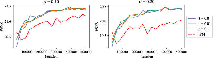
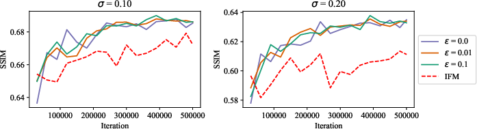
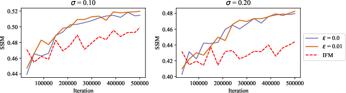
- What: Use condition-preserving triangular maps with SD-FM (augmented cost c((x, z), (x′, z′)) = cX(x, x′) + β cZ(z, z′)) for class-conditional and continuous conditions, demonstrated on ImageNet classes and super-resolution (CelebA, 4×/8×) with improved PSNR/SSIM.
- Tools/workflow:
- Build SD-OT on the augmented (x, z) space; tune β; reuse the same g during FM training.
- For super-resolution, condition on low-res/noisy images; deploy as a fast enhancement module.
- Assumptions/dependencies:
- Condition embeddings are well-calibrated (β scaling matters).
- For continuous z, costs must reflect task geometry; pairing quality hinges on c and ε.
- Low-NFE generation and on-device viability via straighter flows
- Sector: Mobile/Edge AI, Creative Apps, AR/VR
- What: SD-FM reduces flow curvature, enabling fewer ODE NFEs (Euler/Dopri) while preserving quality. This lowers latency and energy, supporting on-device or low-end GPU inference.
- Tools/workflow:
- Swap independent coupling with SD-FM during training; keep inference stack unchanged.
- Assumptions/dependencies:
- Benefit correlates with pairing quality (tracked by χ²); precompute g once per dataset/task.
- One-step and few-step generation improvements for consistency/mean-flow models
- Sector: Software/AI, Media/Creative
- What: Apply SD-OT couplings to MeanFlow (and related consistency training) to improve one-step generation quality for latent or pixel-space models (e.g., DiT-XL/2 latent ImgN-256).
- Tools/workflow:
- Train consistency-style models with SD-FM pairing; combine with existing schedulers.
- Assumptions/dependencies:
- Same as SD-FM; larger benefits where trajectory consistency is crucial.
- Corrected guidance for controllable generation (classifier-free/autoguidance)
- Sector: Media/Creative, Design Tools, Advertising
- What: Use the generalized Tweedie formula to compute scores from SD-FM velocity fields (ε≈0 or ε→∞) and apply the paper’s resampling-based “corrector” to sample from the intended geometric mixture ργ ∝ ργ
- 1 ρ1−γ
- 2, thus improving faithfulness of guided generations.
- Tools/workflow:
- Generate r parallel trajectories with mixed velocity field; reweight by the provided integral of velocity-score differences; select a trajectory via softmax over weights.
- Assumptions/dependencies:
- Extra compute for r trajectories; ε small or infinite to use velocity-to-score link; best suited for “hero” renders or batch selection.
- Cost- and energy-efficient precompute vs. OT-FM for small/medium labs
- Sector: Academia, Startups/SMBs, Cloud ML
- What: Replace multi-node Sinkhorn pipelines with single-node SD-OT SGD to obtain OT-quality couplings without quadratic n/ε scaling; democratizes OT-guided FM.
- Tools/workflow:
- Adopt ott-jax SD-OT; monitor unbiased χ² to stop precompute; cache g per dataset.
- Assumptions/dependencies:
- Requires a single multi-GPU node for large N; pairing can be amortized or ANN-accelerated.
- Dataset-specific “pairing index” for reproducible training
- Sector: MLOps/Tooling
- What: Cache the dual potential vector g as a dataset artifact; reuse across ablations/hyperparam sweeps and different network architectures to standardize the coupling used for FM.
- Tools/workflow:
- Store g with dataset versioning; expose MIPS service to training jobs.
- Assumptions/dependencies:
- g is dataset- and cost-specific; significant distribution shift requires re-fitting.
- Monitoring and validation with the unbiased χ² marginal criterion
- Sector: Academia, MLOps/Tooling
- What: Track convergence of SD-OT via the proposed unbiased χ² estimator (O(NB)); detect underfitting or over-regularization (ε, β).
- Tools/workflow:
- Add χ² to training dashboards; schedule early stopping or ε-tempering.
- Assumptions/dependencies:
- Requires batches from the noise distribution during precompute; estimator variance decreases with batch size.
- Photography and communication apps: robust super-resolution
- Sector: Consumer Apps, Telecom/Video Conferencing
- What: Improved 4×/8× SR under noise (σ=0.1/0.2) with SD-FM conditioning; deploy for photo enhancement and bandwidth-limited video upscaling.
- Tools/workflow:
- Train SR models with SD-FM; export compact inference graphs (few NFEs).
- Assumptions/dependencies:
- Quality hinges on condition cost and ε; device constraints may favor small models and ε=0.
- Documentation and compute reporting for sustainable AI
- Sector: Policy/Standards, Corporate ESG
- What: Standardize reporting of precompute vs. training/inference budgets; show SD-FM’s energy savings compared to OT-FM while improving quality.
- Tools/workflow:
- Add a “pairing overhead per-sample” metric alongside NFEs and FID/PSNR/SSIM.
- Assumptions/dependencies:
- Organizational buy-in; comparable baselines across teams.
Long-Term Applications
These require further research, scaling, or engineering to reach production robustness.
- Web-scale SD-FM with billion-sample datasets
- Sector: Foundation Models, Cloud ML
- What: Shard SD-OT across nodes, approximate/multi-stage ANN for MIPS, and hierarchical potentials to extend to N ≫ 108.
- Potential tools/workflow:
- Hierarchical Laguerre cell indexing; vector DBs; streaming/online g updates with χ² monitoring.
- Assumptions/dependencies:
- Robust distributed ANN; memory and I/O optimized storage of g; stability under dataset churn.
- On-device and federated personalization using semidiscrete couplings
- Sector: Mobile/Edge AI, Privacy-Preserving ML
- What: Fit g on-device over a user’s private gallery and SD-FM train a personalized generator with minimal cloud compute; pair noise to local exemplars via MIPS.
- Potential tools/workflow:
- On-device SD-OT SGD with ε=0; secure ANN; federated aggregation of model deltas (not data).
- Assumptions/dependencies:
- Limited on-device compute; privacy and consent; small-N regimes need regularization/tempering.
- Cross-modal and domain-adaptation SD-FM (text-image, audio, 3D, robotics sim2real)
- Sector: Multimodal AI, Robotics
- What: Use cross-modal costs (e.g., CLIP-like embeddings) or task-tailored costs in SD-OT to better align noise with data across domains (e.g., sim observations to real sensory data).
- Potential tools/workflow:
- Embed both sides into a shared space for dot-product costs; extend generalized Tweedie for non-Gaussian ρ0.
- Assumptions/dependencies:
- Well-behaved cross-modal embeddings; careful β scaling; theoretical extensions beyond Gaussian source.
- Retrieval-augmented FM: curriculum and class-balance via potentials
- Sector: MLOps/Tooling, Fairness
- What: Use g and Laguerre cells to modulate sampling curriculum, balance long-tail classes, or debias pairings; integrate with active learning.
- Potential tools/workflow:
- Weighting or gating by cell occupancy; priority queues for rare regions.
- Assumptions/dependencies:
- Correlation between pairing structure and fairness goals; monitoring for unintended bias.
- Data curation and deduplication signals from SD-OT
- Sector: Data Engineering, Compliance
- What: Analyze potentials and cell structure to detect duplicates, outliers, and underrepresented clusters; guide dataset pruning or augmentation.
- Potential tools/workflow:
- Visualization of Laguerre partitions; pairwise audit trails from MIPS matches.
- Assumptions/dependencies:
- Interpretability of g; linkage between partition geometry and data quality.
- Provable, resource-aware guided sampling for high-stakes generation
- Sector: Media/Creative, Enterprise Content
- What: Productionizable correctors that approximate mixture targets ργ with adaptive r and early stopping; allocate more r only when needed.
- Potential tools/workflow:
- Online estimation of the reweighting integral; bandit-style allocation of trajectories.
- Assumptions/dependencies:
- Stable velocity-to-score mapping under ε≈0; user tolerance for variable latency.
- Safety and governance via pairing constraints
- Sector: Policy/Safety
- What: Impose constraints in SD-OT pairing (e.g., forbid matches to sensitive exemplars) to steer training away from restricted content and improve traceability.
- Potential tools/workflow:
- Masked MIPS; policy-aware costs (penalize restricted regions).
- Assumptions/dependencies:
- Reliable content filters/labels; maintaining model quality under constraints.
- Generalized Tweedie beyond Gaussian sources and broader guidance theory
- Sector: Academia
- What: Extend the score–velocity identity to other sources/interpolants; build theory and practical correctors for complex guidance stacks and multi-condition mixtures.
- Potential tools/workflow:
- New interpolants with analytic score links; numerical studies on variance/efficiency of resampling schemes.
- Assumptions/dependencies:
- Additional regularity; new proofs akin to the paper’s ε→0/∞ analysis.
- Standardization of compute–quality trade-offs for green AI
- Sector: Policy/Standards, ESG
- What: Introduce benchmarks that include “pairing overhead per-sample,” χ² at convergence, and total energy for coupling + training + inference; inform procurement and emission reporting.
- Potential tools/workflow:
- Shared leaderboards with compute metrics; LCA (life-cycle assessment) of training pipelines.
- Assumptions/dependencies:
- Cross-organization cooperation; reliable metering.
Notes on key assumptions and dependencies across applications
- Semidiscrete setting: target dataset is finite (size N). Gains hinge on learning a good dual potential g; quality can be tracked by the unbiased χ² divergence (smaller is better, saturation observed around practical thresholds).
- Costs and ε: dot-product cost is favored for speed and MIPS; ε≈0 enables hard assignments and fast ANN; ε>0 entails softmax sampling and higher per-step cost but can be useful for smoothing.
- Scalability: MIPS/ANN is the main systems dependency; PCA or learned projections can reduce dimensionality for pairing without altering the FM architecture.
- Theory: The ε=0 convergence guarantees rely on regularity (density of μ, minimal separation δ between data points, bounded surface area measure); practice often uses ε≈0 with strong empirical gains.
- Reuse: g is dataset-dependent but architecture-agnostic; once precomputed, it can be reused across model sizes and ablations, amortizing cost.
Glossary
- Autoguidance: A guidance technique that combines models by weighting their velocity fields to steer sampling toward preferred outputs. "or, more generally, autoguidance \citep{karras2024guiding}, where ρ_2 is a weaker model compared to ρ_1."
- Benamou–Brenier least-action principle: An OT-based formulation viewing transport as a minimal kinetic energy (least-action) flow connecting two distributions. "motivated by the dynamic least-action principle of \citeauthor{benamou2000computational}."
- Categorical sampling: Drawing an index from a discrete probability distribution over classes or items. "for , this amounts to a categorical sampling among points"
- Classifier-free guidance (CFG): A generative guidance method that mixes conditional and unconditional models to trade off fidelity and diversity. "One example is classifier-free guidance \citep{ho2022classifier} where is a conditional model and is unconditional"
- Consistency models: Generative models trained with objectives enforcing consistency across trajectories or time steps, enabling few-step sampling. "Recently, consistency models (models that incorporate trajectory consistency constraints in their training objective) have become a popular choice for few-step generation with diffusions or flows"
- Entropic regularization: A smoothing term added to OT objectives that encourages high-entropy couplings and enables efficient algorithms. "defined for two probability measures , a cost function and entropic regularization as:"
- Flow curvature: A measure of how bent or non-straight the ODE trajectories are; lower curvature typically eases numerical integration. "We measure generation quality using FID~\citep{heusel2017gans} and flow curvature \citep{lee2023minimizing}."
- Flow matching (FM): A training method that aligns a time-dependent velocity field with target displacements along interpolated segments, avoiding backpropagation through ODE solvers. "Flow models parameterized as time-dependent velocity fields~\citep{chen2018neural} can be efficiently trained using flow matching (FM)"
- Hungarian algorithm: A polynomial-time method for solving linear assignment problems that finds optimal matchings between sets. "e.g. the Hungarian algorithm,~\citealt{kuhn1955hungarian}"
- Kullback–Leibler divergence (KL): A measure of dissimilarity between probability distributions, often used as a regularizer in OT. "+ \varepsilon KL(\pi | \mu\otimes\nu),"
- Laguerre cells: Generalized Voronoi regions arising in semidiscrete OT that partition space based on affine scores tied to dual potentials. "Laguerre cells~\citep{merigot2011multiscale} being illustrated in the plot."
- Maximum inner product search (MIPS): The problem of finding, for a query vector, the dataset vector with the largest dot product, often used for fast matching. "at the cost of a maximum inner product search (MIPS) over the dataset."
- MeanFlow (MF): A consistency-style flow model designed for few-step or one-step generation via mean-field objectives. "We demonstrate that the benefits of SD-OT couplings go beyond FM by testing them on the MeanFlow (MF) model of \citet{geng2025mean}"
- Monge map: The deterministic transport map that pushes one distribution to another while minimizing a given cost, central in OT. "That map is exactly the \citeauthor{Monge1781} map"
- Number of function evaluations (NFEs): The count of neural function calls needed by an ODE solver to integrate trajectories; a key inference cost metric. "In practice, the quality of samples is highly dependent on the number of function evaluations (NFEs) used to integrate the ODE."
- Optimal transport (OT): A mathematical framework for moving probability mass from one distribution to another at minimal cost. "matching batches of noise to target points using an optimal transport (OT) solver."
- Probability flow ODE: An ordinary differential equation whose velocity field transports a source distribution to a target distribution along a continuous probability path. "That interpolant can be written equivalently as a probability flow ODE"
- Pushforward operator: The operation that maps a distribution through a function, producing the distribution of the transformed random variable. "where , where is the pushforward operator"
- Semidiscrete optimal transport (SD-OT): An OT setting where one measure is continuous and the other is discrete, solved via dual potentials and often SGD. "We leverage the entropy regularized semidiscrete (SD) formulation of OT"
- Semidual (formulation): A dual optimization formulation of OT that reduces to maximizing over potentials on the discrete support. "This problem can be written in a semidual form"
- Sinkhorn algorithm: An iterative scaling method for computing entropically regularized OT couplings efficiently. "using a multi-GPU-node implementation of the \citeauthor{Sinkhorn64} algorithm"
- Soft-c transform: A transformation mapping inputs to smoothed costs via log-sum-exp (or max) over discrete supports, central in SD-OT. "we define the soft- transform ~\citep[\S5.3]{PeyCut19} as:"
- Triangular maps: Structure-preserving transport maps that leave conditioning variables unchanged while transforming data conditioned on them. "condition-preserving triangular maps "
- Tweedie formula: A relationship connecting posterior means to gradients of log densities (scores), used to link velocity and score estimation. "We propose a generalization of the Tweedie formula"
Collections
Sign up for free to add this paper to one or more collections.

