No Validation, No Problem: Predicting Model Performance from a Single Gradient
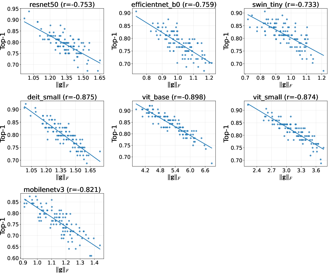
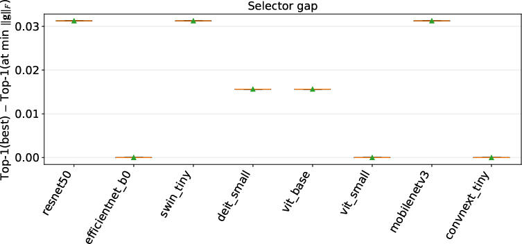
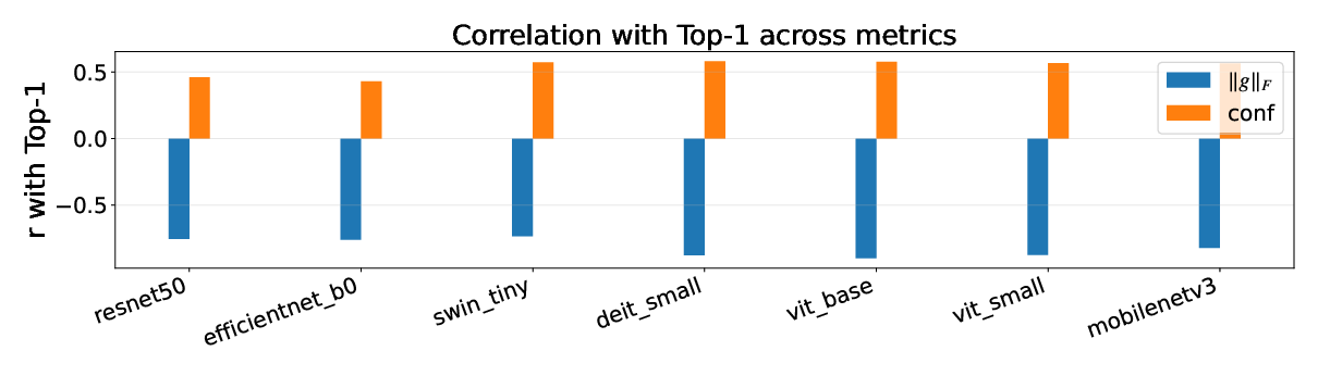
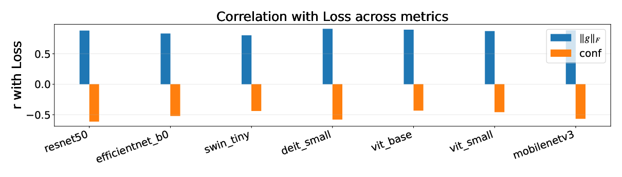
Abstract: We propose a validation-free checkpointing signal from a single forward-backward pass: the Frobenius norm of the classifier-head gradient on one detached-feature batch, ||g||_F = ||dL/dW||_F. Across ImageNet-1k CNNs and Transformers, this proxy is strongly negative with Top-1 and positive with loss. Selecting the checkpoint with the minimum head gradient in a short tail window closes most of the gap to the oracle (4.24% +/- 2.00% with a universal setup, about 1.12% with light per-family tuning). For practical deployment, a head-scale normalization is more stable within classic CNN families (e.g., ResNets), while a feature-scale normalization works well for Transformers and modern CNNs. The same one-batch probe also predicts COCO detection/segmentation mAP. In diffusion (UNet/DDPM on CIFAR-10), it tracks progress and enables near-oracle tail-window selection; it is positively correlated with same-distribution probe MSE and negatively with FID (lower is better), so it can be used as a lightweight, label-free monitor. Validation labels are never used beyond reporting. The probe adds much less than 0.1% of an epoch and works as a drop-in for validation-free checkpoint selection and early stopping.
Paper Prompts
Sign up for free to create and run prompts on this paper using GPT-5.
Top Community Prompts
Explain it Like I'm 14
What this paper is about (big idea)
Training AI models usually needs a “validation set” to check how good the model is and decide when to stop or which version (“checkpoint”) to keep. That takes extra time and labeled data. This paper shows a surprising shortcut: you can predict how good a model is using just one tiny batch of data and one quick calculation of how much the model’s last layer wants to change. If that “change size” is small, the model is usually doing well; if it’s big, the model is usually doing worse.
What questions the paper asks
- Can we tell how good a model is without using a validation set, using only:
- one small batch of data
- one forward pass and one backward pass (a single “backprop”)?
- Does this simple score work across different tasks, like:
- Image classification (e.g., ImageNet)
- Object detection and instance segmentation (e.g., COCO)
- Image generation with diffusion models (e.g., CIFAR-10)?
- Can this score pick the best checkpoint during training (early stopping) almost as well as the usual “oracle” that uses the full validation set?
- Is it cheap and simple enough to drop into real training pipelines?
How the method works (in everyday language)
Think of a deep model as two parts:
- A feature extractor (turns an image into a useful set of numbers)
- A simple “head” (usually a linear layer) that turns those numbers into a final answer (like which class an image belongs to)
The paper looks at the head only and asks: “If we took one small batch of data and told the head to improve, how much would it want to change?” That “how much” is measured by a single number: the size (norm) of the head’s gradient. The steps are:
- Run the model on one small batch to get features.
- “Detach” the features (freeze them) so only the head is allowed to change.
- Compute the usual training loss on that batch (e.g., cross-entropy for classification).
- Backpropagate only through the head to get its gradient.
- Measure the size of that gradient (the Frobenius norm; you can think of it like the overall “length” of all the changes it wants to make).
- Use that single number as the score.
Intuition:
- If the features are already very helpful, the head doesn’t need to change much → small gradient → model likely good.
- If the features aren’t very helpful yet, the head wants to change a lot → big gradient → model likely worse right now.
Two small tweaks make the score fair across different models:
- Feature-scale normalization: divide by the size of the features (works well for Transformers and modern CNNs).
- Head-scale normalization: divide by the size of the head’s weights (works well within classic CNN families like ResNet).
Cost:
- It’s extremely cheap: one tiny extra step that adds far less than 0.1% of an epoch.
What they found and why it matters
Across tasks, a single-batch head-gradient score tracks real performance surprisingly well.
Image classification (ImageNet-1k):
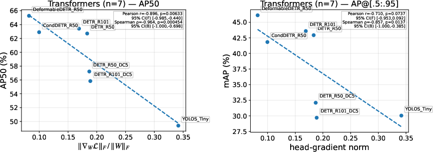
- Lower head-gradient score strongly lines up with higher Top-1 accuracy and lower loss for both CNNs and Transformers.
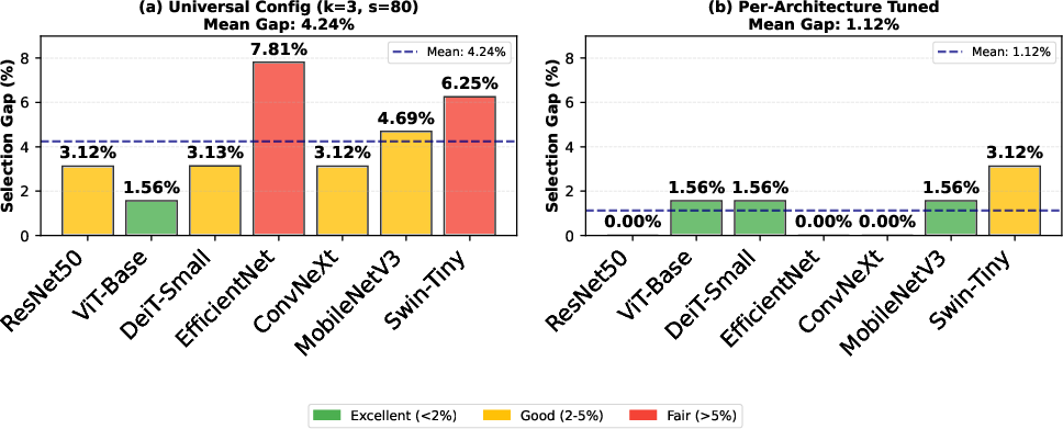
- Picking the checkpoint with the smallest head-gradient score near the end of training closely matches the best validation checkpoint:
- With one universal setting, the average gap is small (roughly a few percent in accuracy).
- With light tuning per model family, the gap shrinks to about ~1% on average.
- This makes early stopping and checkpoint selection possible without validation labels.
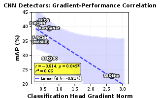
Object detection and instance segmentation (COCO):
- The same one-batch head-gradient idea (applied to the classifier head in detectors) negatively correlates with mAP (mean Average Precision): smaller gradient → better detection and segmentation.
- It works across different detector types (e.g., Faster R-CNN, RetinaNet, Mask R-CNN, Mask2Former, YOLO-Seg).
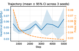
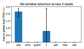
Diffusion models (CIFAR-10 image generation):
- The score tracks training progress and helps choose a good checkpoint near the end.
- It correlates with standard quality measures:
- Positively with the model’s internal probe loss (MSE)
- Negatively with FID (lower FID = better images), meaning higher score tends to mean better image quality here.
- It acts as a label-free, lightweight monitor during training.
Practical perks:
- No validation labels are needed at selection time.
- It’s architecture-agnostic and tiny in compute cost.
- It can pre-screen candidate models in small architecture searches, saving around 60% compute while still keeping the best model in the shortlist.
Why it likely works (simple picture):
- When the model is in a “flatter” and safer spot in its learning landscape, it tends to generalize better. In those spots, the head’s gradient is small. So: smaller head gradient ≈ better generalization and higher accuracy.
What this means (impact and limits)
Impact:
- Training can be faster and cheaper because you don’t need to repeatedly run full validation.
- Helpful when labels are scarce, private, or not available for validation.
- Easy to add to existing training code as a “drop-in” early-stopping and checkpoint-selection tool.
- Useful as a quick, rough filter when comparing models from the same family (e.g., different ResNets) or checkpoints from the same run.
Limits:
- Best for picking checkpoints within one training run or comparing models within the same family.
- Less reliable for ranking very different pretrained backbones across families (e.g., ResNet vs. ViT) for a new dataset; in that case, the cross-family ranking can break down.
- Unusual training setups (very tiny or huge batches, heavy regularization) may need small adjustments (like the normalizations mentioned above).
Takeaway
A single, tiny test—measuring how much the last layer wants to change on one small batch—can reliably tell you how good your model is, without using a validation set. It’s simple, fast, and works across classification, detection, segmentation, and even diffusion models. This can cut training costs, simplify early stopping, and make model selection much easier in practice.
Knowledge Gaps
Knowledge gaps, limitations, and open questions
Below is a consolidated list of unresolved issues that are either missing, uncertain, or left unexplored in the paper; each item is phrased to be directly actionable for follow-up research.
- Cross-domain generality: Validate whether a single-batch head-gradient proxy extends beyond vision to NLP (e.g., language modeling, sequence classification), speech, graphs, and reinforcement learning, especially for models without an explicit linear “classification head.”
- Transfer learning across heterogeneous families: The paper reports collapse in cross-family pretrained→transfer ranking. Investigate normalization, calibration, or lightweight adaptation strategies (e.g., re-centering features, per-family scaling, shallow adapters) that enable reliable cross-family selection on downstream tasks.
- OOD and distribution shift robustness: Quantify how well the proxy predicts performance under dataset shift (e.g., ImageNet-V2/-A/-R, ImageNet-C, COCO-OOD subsets, domain adaptation settings), and whether batch selection from target vs source distributions changes reliability.
- Truly label-free classification selection: The current classification probe requires labels for cross-entropy. Develop and evaluate unsupervised variants (e.g., entropy-based losses, pseudo-labels, self-supervised/contrastive heads) that preserve predictive power without any labels.
- Batch sensitivity and sampling strategy: Characterize variability across different probe batches (size B, class mix, rare classes, imbalance). Estimate the minimal batch size for stable ranking, propose robust aggregation (e.g., K batches with trimmed mean/median), and provide CIs for selection decisions.
- Training/eval mode and stochastic layers: Establish best practices for BatchNorm/LayerNorm/Dropout during probing (train vs eval mode), ensure running stats are not altered, and quantify the impact of these choices on the proxy.
- Sensitivity to training tricks: Systematically study effects of label smoothing, temperature scaling, Mixup/CutMix, knowledge distillation, stochastic depth, weight averaging/EMA, and data augmentation policies on the correlation and selection gap.
- Optimizer and regularization dependence: Assess robustness across optimizers (SGD+momentum, Adam/AdamW, Adafactor), schedules (cosine, step, warmup), and regularization (decoupled weight decay, SAM). Determine if head- or feature-normalizations fully remove optimizer-induced scale confounds.
- Nonlinear and multi-layer heads: The method assumes a linear head. Evaluate how to define the proxy for MLP heads, normalized or weight-tying heads, and whether to probe the last layer only or aggregate over layers.
- Multi-label and long-tail classification: Extend and validate the proxy under BCE losses, class imbalance, and long-tail distributions; test calibration for per-class vs overall performance.
- Multi-task settings: For detectors/segmenters with multiple heads, compare using classification-head-only gradients versus combining gradients from localization/regression/mask heads; study which combination best predicts mAP/AP.
- Detection assignment fidelity: Replace the simplified IoU>0.5 nearest assignment with each detector’s native assignment (Hungarian, ATSS, etc.) during probing and quantify the resulting change in correlation and sample efficiency.
- Instance/semantic/panoptic segmentation breadth: Expand beyond 12 models to larger, more diverse segmenters (including semantic and panoptic) and compare gradients from classification vs mask heads to determine the most predictive probe.
- Normalization choice automation: Provide a principled, model-agnostic rule (or learned selector) to choose between feature-scale and head-scale normalizations (or a combined invariant metric), removing the need for per-family heuristics.
- Early-stopping hyperparameters without labels: Develop a label-free scheme to set tail-window size, EMA span, quantile, and patience automatically, with guarantees on expected selection gap.
- Theoretical grounding: Formalize conditions under which the detached head-gradient norm is monotonic with generalization (e.g., links to margin/linear separability, Fisher information, sharpness bounds), and characterize failure modes.
- Scalability to very large heads: Measure compute/memory overhead and reliability for extremely large output spaces (e.g., ImageNet-22k, wordpiece vocabularies in LMs), and propose memory-efficient approximations if needed.
- Diffusion generalization: Validate on higher-resolution and conditional diffusion (class-conditional, text-to-image latent diffusion), alternative parameterizations (v-prediction), guidance strengths, schedulers (DDPM, DDIM, DPM-Solver, EDM), and timestep sampling policies (probe across t∈[0,T] vs restricted ranges).
- Probe-time timestep policy in diffusion: Justify and test the choice t∼Uniform([0.1T,0.7T]); evaluate correlations when probing early/late noise scales, and whether a weighted or learned t-schedule improves stability.
- Robustness to gaming and adversarial batches: Study whether one can “cherry-pick” or adversarially craft probe batches to manipulate selection, and design defenses (randomized batching, outlier rejection, bagging).
- Privacy and DP constraints: If labels are private, evaluate whether the single-batch gradient norm can be computed under differential privacy (DP-SGD) with acceptable noise and still retain predictive power.
- Checkpoint cadence and sparsity: Analyze how probe frequency and checkpoint sparsity affect selection gap, and whether interpolation or adaptive probing schedules can reduce compute while preserving accuracy.
- Mapping score to predicted accuracy: Move beyond ranking to calibrated accuracy/mAP prediction with uncertainty estimates, enabling downstream scheduling or resource allocation decisions.
- Early-phase predictivity: Test whether the proxy measured early in training can forecast final performance (useful for early termination), and compare against learning-curve extrapolation baselines.
- Standard NAS benchmarks: Evaluate the method as a pre-screen on NAS-Bench-201/NATS-Bench (using trained or partially trained checkpoints) to quantify recall@K and compute savings versus established zero-cost proxies.
- Distributed training effects: Specify and test how to compute the probe under DDP (synchronized BN, gradient reduction), ensuring no interference with training states and reproducibility across nodes.
- Per-class/feature whitening: Explore more invariant normalizations (e.g., whitening Z, per-class scaling, Fisher-normalized gradients) to mitigate feature/weight scale confounds and improve cross-architecture comparability.
- Few-shot and low-resource regimes: Validate stability and utility when only a handful of labeled samples are available for probing, including class-balanced vs imbalanced few-shot splits.
- Wider dataset coverage: Extend evaluations to additional benchmarks (e.g., VTAB, WILDS, ImageNet-Real, ADE20K, Cityscapes, OpenImages) to test external validity across tasks and data regimes.
Practical Applications
Immediate Applications
The following items summarize practical, deployable uses of the paper’s single-batch, head-only gradient probe for validation-free checkpoint selection and monitoring. Each item notes relevant sectors, potential tools/workflows, and key assumptions.
- Validation-free early stopping and checkpoint selection in supervised vision training
- Sectors: software (MLOps), healthcare (medical imaging classifiers), robotics (perception models), finance (document/image classification).
- Tools/workflows: PyTorch/Lightning callback that computes min g² or normalized scores in a tail window; MLflow/W&B integration to log g² and auto-select checkpoints; CI/CD training pipelines with periodic gradient probes instead of full validation passes.
- Assumptions/dependencies: supervised training with a standard classifier head; uses one labeled training batch; feature/head-scale normalization chosen appropriately (feature-scale for Transformers/modern CNNs; head-scale for classic CNNs like ResNet); tail-window selection and light EMA smoothing; batch-size-insensitive reduction (mean) recommended.
- Label-free monitoring for diffusion models (UNet/DDPM)
- Sectors: media and entertainment (image generation), advertising, gaming, design tools.
- Tools/workflows: training dashboard metric derived from head-gradient MSE probe; tail-window checkpoint selection using EMA-smoothed score_w; alerting when gradient trends deviate.
- Assumptions/dependencies: no validation labels required; probe uses the native MSE loss on a fixed set of images and timesteps; gradient computed on the noise-prediction head only; correlation is negative with FID and positive with probe MSE.
- Lightweight, in-family NAS-style pre-screening of trained or partially trained candidates
- Sectors: software (AutoML), robotics (perception model selection), healthcare (model variant selection), edge AI (resource-constrained deployments).
- Tools/workflows: “pre-screen” stage in NAS/AutoML pipelines that ranks family-specific candidates by min g²/score_w/score_z before expensive fine-tuning; high-recall K-of-N shortlist to cut compute.
- Assumptions/dependencies: reliable within-family ranking (e.g., ResNet variants); not robust across heterogeneous families; consistent training recipe across compared candidates.
- Compute and energy savings in production training loops
- Sectors: energy and sustainability, cloud providers, enterprise MLOps.
- Tools/workflows: replace frequent full validation passes with a single-batch gradient probe; auto-stop or checkpoint selection when min g² is reached; report saved FLOPs and emissions in training reports.
- Assumptions/dependencies: minimal added FLOPs/memory (head-only backward pass); organization accepts proxy-based checkpoint selection; periodic validation still possible for auditing/reporting.
- Privacy-aware training pipelines without held-out labeled validation
- Sectors: healthcare (HIPAA), finance (GDPR/CCPA compliance), public sector.
- Tools/workflows: train on labeled data but avoid collecting/using separate validation labels; use gradient probe for selection/early stopping; compliance documentation showing validation-free selection.
- Assumptions/dependencies: supervised training labels available for the probe (one batch); governance accepts validation-free selection for deployment decisions.
- On-device and edge fine-tuning with tight compute budgets
- Sectors: mobile, IoT, robotics.
- Tools/workflows: on-device early stopping via a single-batch head-gradient probe to minimize validation overhead; local checkpoint selection with few steps.
- Assumptions/dependencies: small memory footprint for head grads/logits; simple classifier head; one small labeled batch available or synthetic labels in constrained cases.
- Academic experimentation efficiency and reproducibility
- Sectors: academia, education.
- Tools/workflows: use g² curves to track progress across runs; fewer validation passes in hyperparameter sweeps; publish gradient-probe logs alongside results.
- Assumptions/dependencies: conventional supervised setups and heads; standard correlation trends hold under common training regimes; document smoothing/window choices.
- Instance segmentation and object detection model selection without full validation
- Sectors: retail (inventory vision), autonomous systems, smart cities.
- Tools/workflows: compute classification-head gradient norm using native assignment rules (IoU/ATSS/Hungarian) on small training batches; rank detectors/segmenters by the probe; deploy best-performing candidate.
- Assumptions/dependencies: probe applied to classification head only; consistent assignment rule; results strongest for AP50 and remain reliable with modest evaluation subset sizes.
Long-Term Applications
These opportunities require further research, scaling, or development to reach broad reliability across tasks and domains.
- Cross-family architecture ranking and transfer selection
- Sectors: AutoML, foundation model deployment across domains.
- Tools/workflows: develop robust scale normalizations or meta-calibrations to compare heterogeneous backbones (ResNet vs. ViT vs. ConvNeXt); integrate into end-to-end NAS frameworks.
- Assumptions/dependencies: current method unreliable for cross-family pools; needs improved normalization, family-aware calibration, or meta-learned scoring.
- Extension beyond vision: NLP, speech, and RL
- Sectors: software (LLMs), conversational AI, recommendation systems.
- Tools/workflows: apply head-gradient probes to language modeling (LM head), sequence classification, token classification; actor/critic heads in RL for early stopping.
- Assumptions/dependencies: appropriate head definition and loss (cross-entropy, MSE); assess correlation robustness under teacher forcing, label smoothing, or RL instability.
- Adaptive training controllers and self-tuning loops
- Sectors: cloud MLOps, enterprise training orchestration.
- Tools/workflows: controllers that adjust learning rate, regularization, or patience based on gradient-probe trends; auto-switch between checkpoints; anomaly detection in training runs.
- Assumptions/dependencies: stable probe dynamics under changing hyperparameters; policy design to avoid oscillations; guardrails for unusual regimes (very small/large batches, heavy regularization).
- Label-free variants for supervised settings with scarce labels
- Sectors: healthcare, public-sector datasets, privacy-restricted environments.
- Tools/workflows: use pseudo-labels, self-supervised heads, or confidence-weighted targets to compute probes without labeled data; compare robustness to supervised probe.
- Assumptions/dependencies: accuracy of pseudo-labels; potential bias under class imbalance or distribution shift; validation of correlation strength.
- Distribution shift–aware monitoring and selection
- Sectors: autonomous systems, finance risk modeling, healthcare (new site data).
- Tools/workflows: combine gradient probe with shift detectors; adapt probe batch sourcing to reflect changing data distributions; multi-batch ensemble probes for robustness.
- Assumptions/dependencies: sampling strategy matters; need methods to avoid overfitting to a non-representative batch; uncertainty quantification around probe scores.
- Governance, auditability, and standards for training metrics
- Sectors: policy, compliance, enterprise risk management.
- Tools/workflows: standardize logging of gradient-based training KPIs; auditors review probe trajectories as evidence of model quality trends; include in model cards.
- Assumptions/dependencies: accepted best practices and benchmarks; documented limitations; complementary metrics (confidence/margin, loss) for triangulation.
- Carbon-aware and cost-optimized training orchestration
- Sectors: energy, cloud providers.
- Tools/workflows: schedulers that use gradient probes to minimize redundant validation compute; integrate with carbon intensity forecasts to time validation runs; cost dashboards.
- Assumptions/dependencies: reliable proxy replacing frequent validation; alignment with organizational SLAs and risk tolerance for proxy-based decisions.
- Hardware and framework support for ultra-cheap gradient probes
- Sectors: semiconductor, AI platform engineering.
- Tools/workflows: kernel-level optimizations for head-only backward passes; framework APIs for detached-feature probing; unified telemetry for probes across model families.
- Assumptions/dependencies: consistent head definitions; support for mixed precision and distributed training; careful numerical stabilization (epsilon terms) in normalization.
Notes on Assumptions and Dependencies (common across applications)
- A conventional classifier head (often linear) and standard supervised loss are assumed; tasks without an explicit classification head may need adaptations.
- For classification/detection/segmentation: one labeled training batch is required for the probe; validation labels are not used.
- For Transformers/modern CNNs, feature-scale normalization (score_z) tends to be more stable; for classic CNNs (ResNet), head-scale normalization (score_w) is preferred.
- Extremely small/large batches or unusual regularization may weaken correlations; modest smoothing (EMA) and tail-window selection improve stability.
- Cross-family ranking is currently unreliable; within-family comparisons and within-run checkpoint selection show strong, stable correlations.
Glossary
- Adaptive Training Sample Selection (ATSS): A detector assignment strategy that selects positive/negative samples adaptively during training. "ATSS~\cite{zhang2020atss}"
- AP50: Average Precision computed at a single IoU threshold of 0.50 in COCO evaluation. "AP50 is the COCO metric âAverage Precision at IoU ,â"
- Average Precision (AP): Area under the precision–recall curve, often averaged over classes or IoU thresholds. "mAP (AP@IoU=0.5:0.95)"
- Bootstrap confidence intervals (CIs): Nonparametric intervals derived by resampling to quantify uncertainty in estimates. "We report Pearsonâs and Spearmanâs with nonparametric bootstrap 95\% CIs (10k resamples)."
- COCO (Common Objects in Context): A large-scale dataset for object detection, segmentation, and captioning. "COCO 2017~\cite{lin2014microsoft} with 118k training and 5k validation images."
- Cross-entropy: A loss function for classification measuring divergence between predicted probabilities and true labels. "and the cross-entropy "
- DDIM (Denoising Diffusion Implicit Models): A deterministic sampler for diffusion models enabling faster generation. "sampling for evaluation uses DDIM~\cite{song2022denoisingdiffusionimplicitmodels} with "
- DDPM (Denoising Diffusion Probabilistic Models): A generative modeling framework using iterative denoising of Gaussian noise. "In diffusion (UNet/DDPM on CIFAR-10), it tracks progress and enables near-oracle tail-window selection;"
- DETR (Detection Transformer): An end-to-end object detector that uses transformers and bipartite matching. "DETR-style~\cite{carion2020end,meng2021conditional,zhu2020deformable} classifier."
- Exponential Moving Average (EMA): A smoothing technique that emphasizes recent values to stabilize metrics or weights. "optionally apply an EMA (exponential moving average)~\cite{brown1959exp,roberts1959ewma} to stabilize the trajectory."
- Fisher trace: A scalar derived from the Fisher Information, used as a proxy for curvature or parameter sensitivity. "and Fisher trace~\cite{amari1998natural}"
- FID (Fréchet Inception Distance): A measure of generative image quality comparing feature distributions of real and generated images. "negatively with FID (lower is better)"
- Frobenius norm: A matrix norm equal to the square root of the sum of squared entries; here used on gradients. "the Frobenius norm of the classifierâhead gradient on one detachedâfeature batch, ."
- Hessian: The matrix of second-order partial derivatives of a loss, capturing local curvature. "where is the Hessian at "
- Hungarian matching: An optimization algorithm for assignment problems used to match detections to targets. "Hungarian matching~\cite{kuhn1955hungarian}"
- ImageNet-1k: A standard 1,000-class image classification benchmark dataset. "Across ImageNetâ1k CNNs and Transformers, this proxy is strongly negative with Topâ1 and positive with loss."
- Intersection over Union (IoU): A metric measuring overlap between predicted and ground-truth regions. "AP@IoU=0.5:0.95"
- Linear separability: The property that classes can be separated by linear boundaries in feature space. "producing a signal that directly reflects the linear separability of current features."
- Logits: Raw, unnormalized scores output by a model before applying softmax. "the logits "
- Mean Average Precision (mAP): Mean of AP over multiple IoU thresholds or classes; standard detection metric. "mean Average Precision (mAP)"
- Neural Architecture Search (NAS): Automated method to discover optimal network architectures. "This use is orthogonal to training-free NAS proxies~\citep{zenscore,tenas,nwot,synflow}"
- Pearson correlation (): A statistic quantifying linear correlation between two variables. "We compute Pearson correlation between the head-gradient norm and validation Top-1 (or loss)"
- Probe MSE: The mean squared error measured by a lightweight probe to assess diffusion training progress. "it is positively correlated with the same-distribution probe MSE"
- Recall@K: The probability that the best item is within the top K selections. "recall@K approaches chance."
- Sharpness: The largest eigenvalue of the Hessian, indicating curvature and sensitivity near a solution. " is its maximum eigenvalue (sharpness)"
- Spearmanâs rho (): A rank-based correlation measuring monotonic relationships. "We report Pearsonâs and Spearmanâs "
- SynFlow: A data-agnostic pruning/gradient-flow proxy used in training-free evaluation. "and gradient-flow proxies such as SynFlow~\citep{synflow}."
- Tail window: The final portion of training steps used for stable checkpoint selection. "enables near-oracle tail-window selection;"
- UNet: A convolutional architecture with encoder–decoder and skip connections, used in diffusion models. "In diffusion (UNet/DDPM on CIFAR-10), it tracks progress"
- Vision Transformer (ViT): A transformer-based image model operating on patch embeddings. "ViT-Base/Small~\cite{dosovitskiy2020image}"
- Zen-NAS: A zero-shot NAS approach with Zen-based measures for architecture scoring. "ZenNAS~\citep{zenscore}"
- Zero-cost proxies: Training-free indicators computed near initialization to predict eventual performance. "without (or before) full training using ``zero-cost'' or training-free indicators"
Collections
Sign up for free to add this paper to one or more collections.