Data-Driven Duration Management -- Term Structure Forecasting Using Machine Learning
Abstract: This paper compares different methods for forecasting the term structure of U.S. and European zero-coupon government bonds using both traditional econometric and Machine Learning (ML) approaches. We compare classical models (e.g., Dynamic Nelson-Siegel (DNS) and Principal Component Analysis (PCA)) with different Neural Network (NN) architectures, including those inspired by the classical models, on the U.S. Treasury market and bonds issued by the European Central Bank (ECB). To enhance predictive performance, macroeconomic variables are incorporated. The findings for both markets are separately analyzed and compared. To this end, we propose a robust model evaluation framework combining statistical accuracy metrics - such as RMSE, MAE, and directional accuracy - with the economic relevance of a quantitative bond trading strategy. Results show that NNs consistently outperform traditional models in both forecasting accuracy and portfolio performance. For the U.S., the most effective approach is a direct-forecasting NN that incorporates DNS factors to reduce the dimensionality of zero-rate data and an Autoencoder (AE) to extract macroeconomic features, while for Europe, the optimal model is a factor-based NN using PCA-derived zero-rate factors without the integration of macroeconomic variables. Overall, the paper demonstrates how combining traditional modeling approaches with modern ML techniques and evaluation can improve yield curve forecasts and support applications in fixed-income portfolio construction.
Paper Prompts
Sign up for free to create and run prompts on this paper.
Top Community Prompts
Explain it Like I'm 14
Data-Driven Duration Management: Term Structure Forecasting Using Machine Learning — Explained Simply
1. What is this paper about?
This paper is about predicting how government bond interest rates will change over time. The “shape” of these interest rates across different time lengths (like 3 months, 1 year, 10 years) is called the yield curve. The authors compare old-school methods and modern ML to see which can predict the yield curve better for the U.S. and Europe. They also test whether these predictions actually help manage a bond portfolio in the real world.
2. What questions did the researchers ask?
Here are the main questions they explored:
- Can modern machine learning methods forecast the yield curve more accurately than traditional models?
- Does adding economic information (like inflation and jobs data) improve predictions?
- Do better predictions translate into better investment decisions (measured by a bond strategy that adjusts risk)?
- Are the best methods the same for the U.S. and Europe?
- How can we build a long-enough European dataset for ML when official data starts later than in the U.S.?
3. How did they do the research? (Methods in everyday language)
First, a few simple ideas:
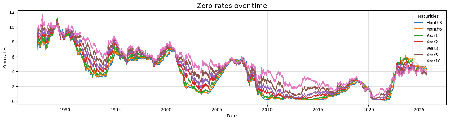
- The yield curve is like a profile of interest rates across different “waiting times” until a bond pays you back—short (months) to long (years).
- A zero-coupon bond is one that pays no regular interest; it just pays a lump sum at the end. The “zero rate” is the interest rate implied by that final payoff.
To handle the complex shape of the curve, the authors use techniques that “compress” the curve into a few summary numbers:
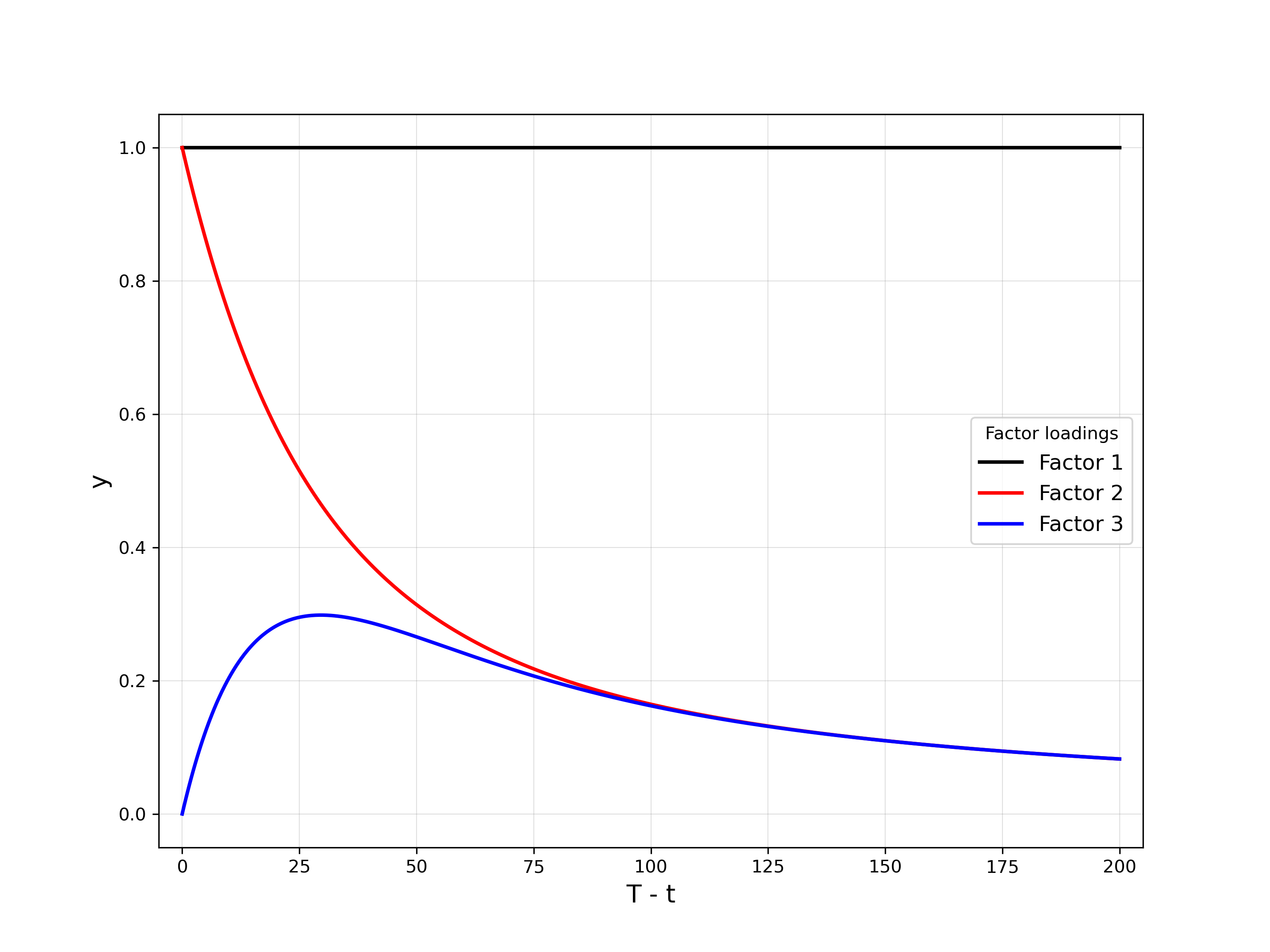
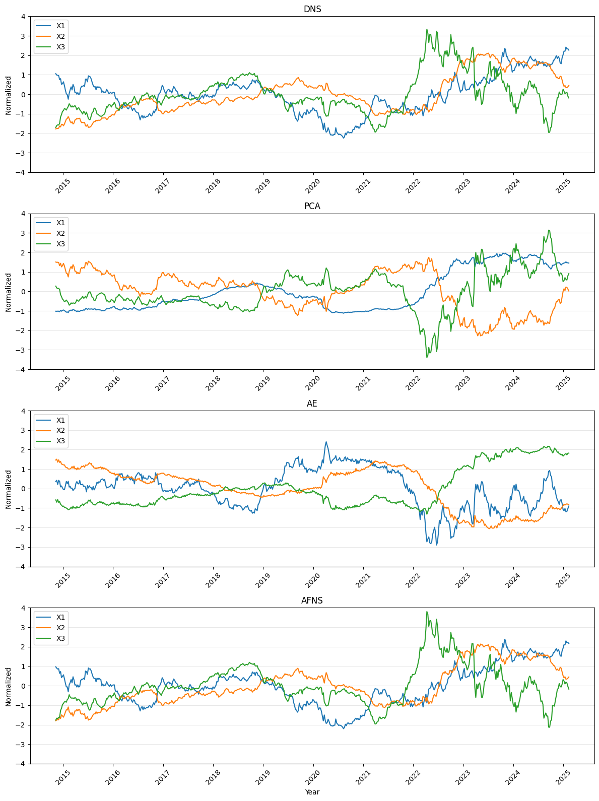
- Dynamic Nelson-Siegel (DNS): A classic model that summarizes the curve into 3 factors:
- Level (overall height of rates),
- Slope (difference between short- and long-term rates),
- Curvature (how “humped” the middle of the curve is).
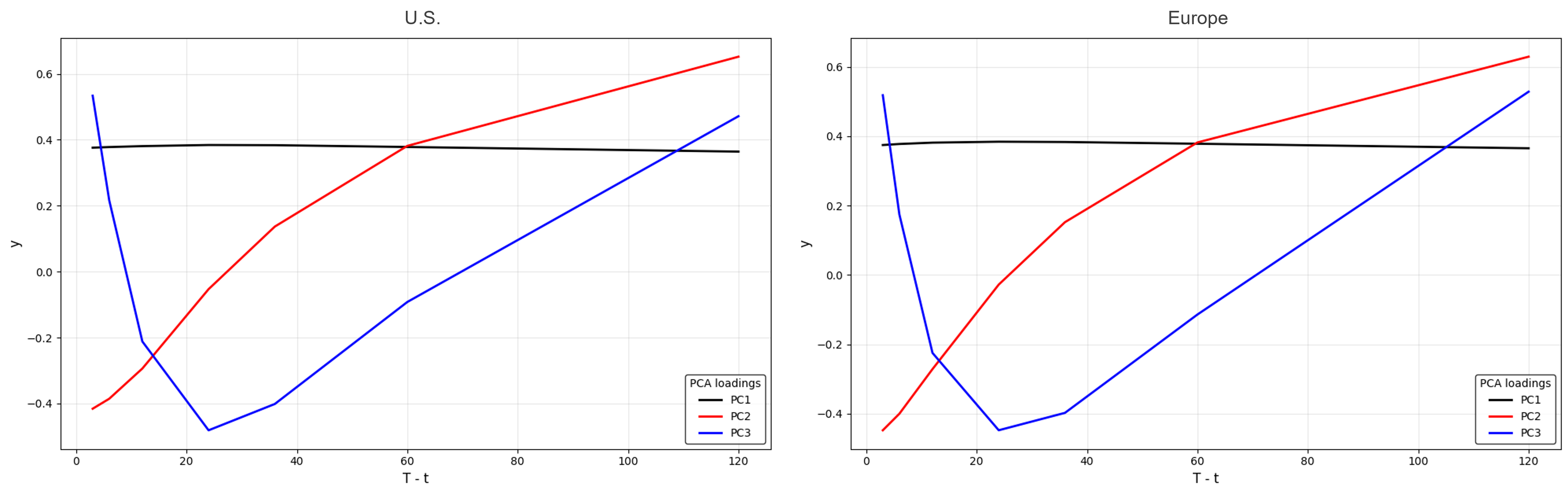
- PCA (Principal Component Analysis): A data-driven way to find 3 main patterns in the curve (which end up acting like level, slope, curvature).
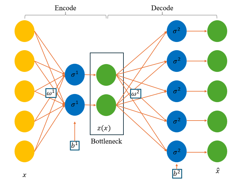
- Autoencoders (AEs): A kind of neural network that learns to compress the curve into a few numbers and then reconstruct it—like a smart photocopier that learns the most important features.
They also consider AFNS (Arbitrage-Free Nelson-Siegel), a version of DNS designed to avoid “free money” opportunities that shouldn’t exist in real markets.
Two main forecasting styles:
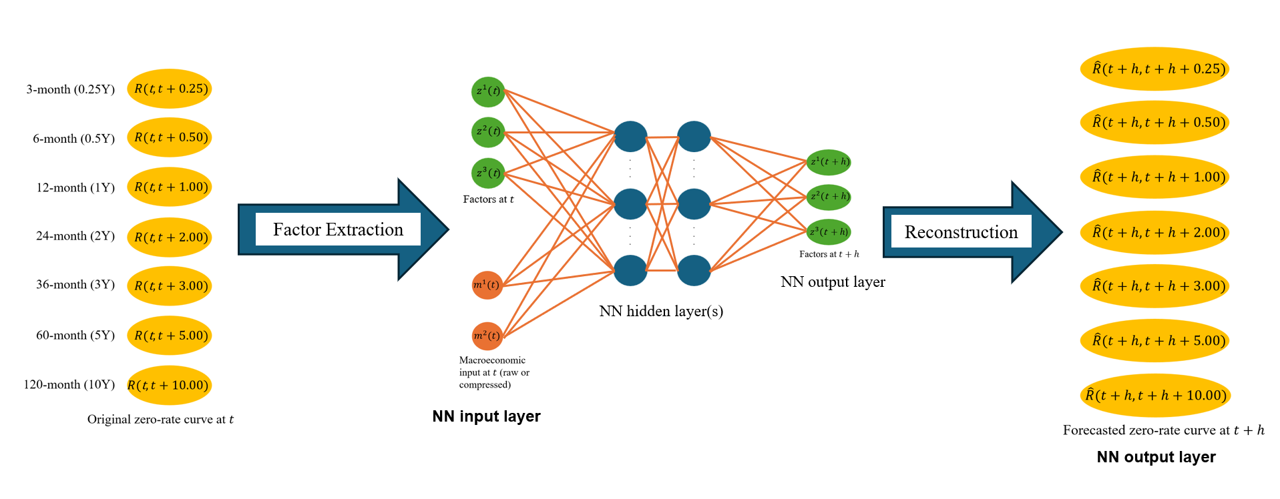
- Factor-based: First compress the curve into 3 factors (using DNS/PCA/AE/AFNS), then predict those factors, and finally rebuild the curve from the predicted factors.
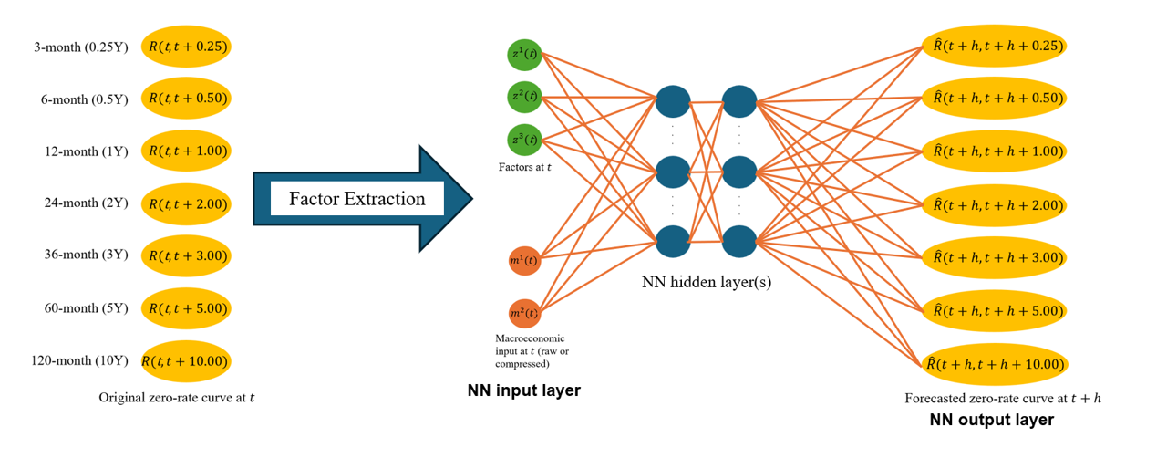
- Direct forecasting: Skip predicting factors. Feed a neural network with today’s factors (or a few chosen rates) and directly predict the full future curve.
Bringing in the economy:
- They add macroeconomic variables: employment, industrial production, inflation (CPI), producer prices (PPI), and a U.S. corporate bond spread (a measure of credit conditions).
- They try using these macro inputs “raw” or “compressed” (using PCA/AE) to see which works better.
Building a stronger European dataset:
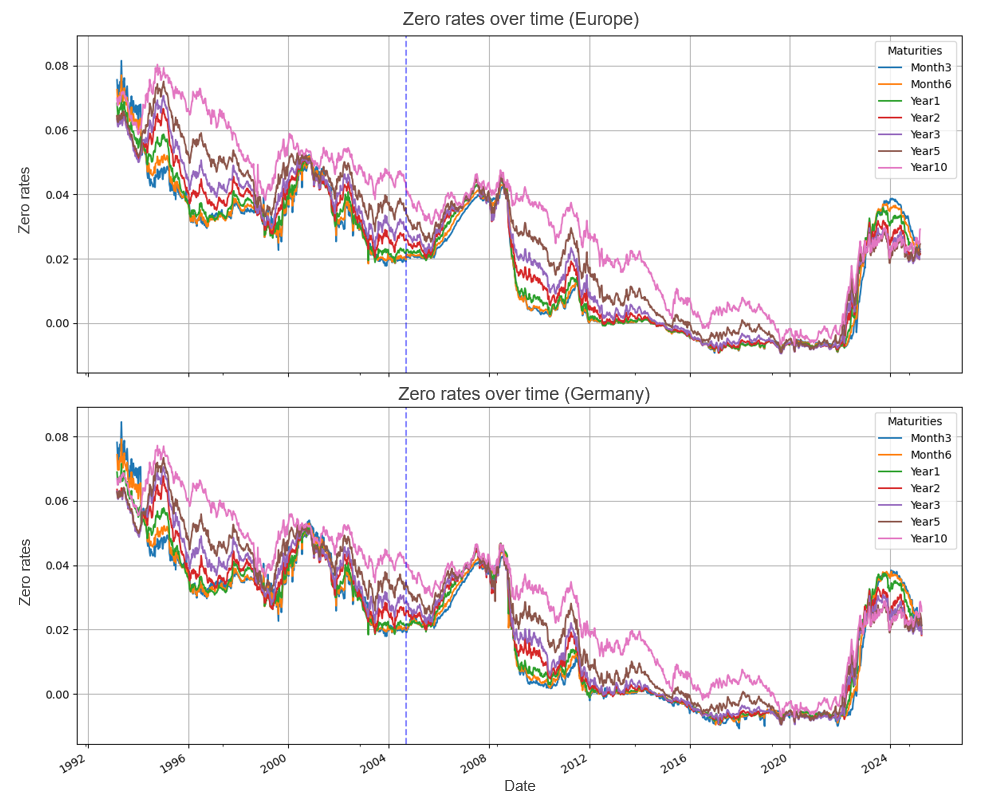
- Problem: Official European Central Bank (ECB) zero-rate data starts in 2004—short for ML.
- Solution: Use German bond data (longer history) as a stand-in. When some German maturities were missing, they filled them in using DNS. Then they learned a tight relationship between German and ECB data in the overlap period and “backcasted” Europe back to 1992. The fit was extremely strong (R² above 0.99), meaning this approach is reliable.
Training and tuning:
- They split the timeline into:
- Training (older data),
- Validation (used to pick the best settings),
- Test (recent years, to measure true out-of-sample performance).
- They re-train from scratch every 2 years (to adapt to big changes) and do small weekly updates (to stay current).
- They use BOHB (a smart search algorithm) to pick model settings like learning rate, network size, and activation functions.
- For robustness, they don’t just chase low error—they also penalize unstable models that make rare but very large mistakes, because those can hurt a portfolio.
Turning forecasts into an investment strategy:
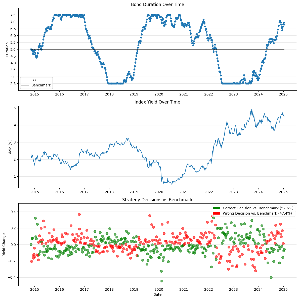
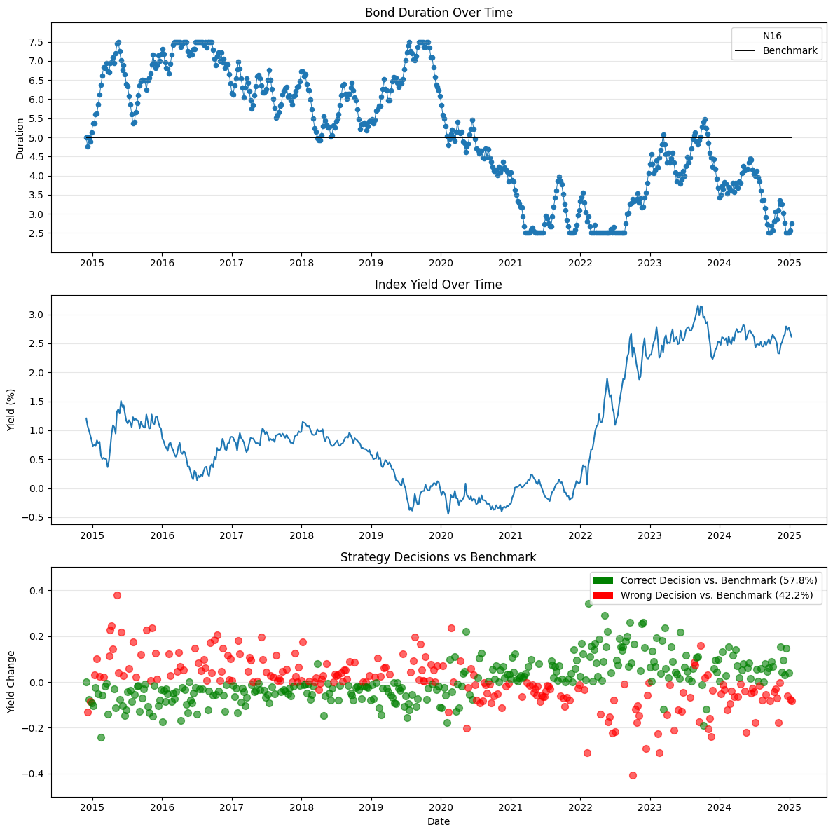
- They use a simple, realistic bond strategy that adjusts “duration,” which measures how sensitive a bond portfolio is to interest rate changes.
- If rates are expected to fall: increase duration (bond prices rise more).
- If rates are expected to rise: decrease duration (protect against losses).
- They predict one month ahead (4 weeks) and update weekly.
- U.S. portfolio: mix of 1-month Treasury bills and a 10-year bond index.
- Europe: similar approach using German bills and a long-term AAA euro government bond index.
- They compare the strategy to a simple passive benchmark (always holding a 5-year duration).
- They judge success by:
- Statistical accuracy (e.g., RMSE, MAE, and getting the direction right),
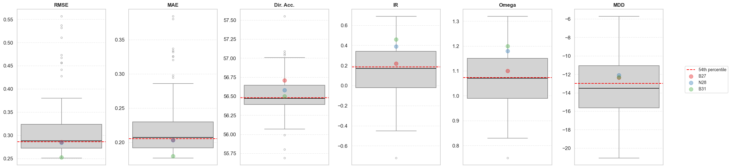
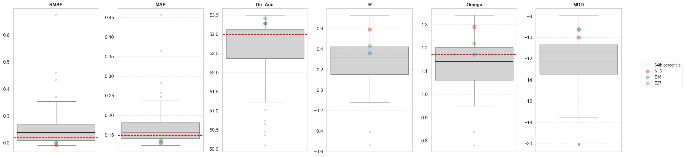
- Investment performance (Information Ratio, Omega Ratio, and Maximum Drawdown).
4. What did they find? (Main results)
Here are the key takeaways:
- Neural networks consistently beat traditional models:
- They were more accurate at forecasting future rates.
- They delivered better portfolio performance (higher risk-adjusted results).
- Best setups differed by region:
- U.S.: The top performer was a direct-forecasting neural network that used DNS factors to summarize today’s yield curve and an autoencoder to summarize macroeconomic data. In other words, compress both the curve and the economy, then predict the future curve directly.
- Europe: The best was a factor-based neural network using PCA factors from the yield curve—without adding macroeconomic variables. In this region, extra macro inputs didn’t help as much.
- The European data-extension method worked very well:
- Backcasting using German data produced highly accurate estimates for the earlier period (R² > 0.99).
- Simpler AEs for the curve worked better than deeper ones:
- A shallower autoencoder (7-3-7) beat a deeper version for curve compression.
- Evaluating both “math accuracy” and “money usefulness” matters:
- Some models with slightly higher errors still gave better trading results, confirming that economic evaluation is essential.
Why this matters:
- More accurate and stable predictions mean better timing when adjusting duration—improving returns and controlling risk.
- The fact that the best model differs between the U.S. and Europe reminds us that markets behave differently, and models should adapt.
5. Why does it matter? (Implications and impact)
- For investors (like pension funds and insurers): Better yield curve forecasts can directly improve how you manage interest rate risk, potentially boosting returns and reducing big losses.
- For researchers and data teams: Combining classic models (DNS/PCA/AFNS) with modern ML creates powerful hybrids: interpretable factors plus flexible neural networks.
- For markets with limited data: The European backcasting approach offers a blueprint for responsibly extending datasets when history is short.
- For real-world decision-making: The paper shows how to judge models not only by prediction error, but by how well they guide actual investment strategies—a more practical and meaningful standard.
- Big picture: Smarter, data-driven duration management can help stabilize portfolios through different interest rate cycles, which matters in a world of fast-changing policy and economic shocks.
In short, the paper shows that modern machine learning—used thoughtfully alongside trusted financial models and tested with real investment rules—can make bond forecasting and portfolio management more effective.
Knowledge Gaps
Knowledge gaps, limitations, and open questions
Below is a single, concrete list of what remains missing, uncertain, or unexplored in the paper that future research could address.
- Data construction risk for Europe: The backcasted Euro area AAA zero rates (pre-2004) rely on a static OLS mapping from German rates with R²>0.99 in-sample; no rolling/regime-specific mapping, stability tests (e.g., Chow/Quandt-Andrews), or uncertainty propagation from the mapping into downstream forecasts are provided.
- Sensitivity to imputation method: Missing German short-maturity data (e.g., 3M/6M/1Y between 1992–1994) are imputed with DNS; the paper shows reconstruction R² but does not quantify how imputation errors affect final forecasts or portfolio performance versus alternative imputation methods (e.g., AFNS/Kalman filter, monotone convex spline, Gaussian process).
- Real-time data and revisions: Macroeconomic inputs use revised series with a fixed 1-month lag and carry-forward; no “real-time” (vintage) data tests, release-lag heterogeneity, or revision-robustness checks are conducted, which may bias ex-ante feasibility and performance.
- Macro coverage and representativeness: The European macro proxy uses German indicators only and omits a corporate spread; this may limit comparability with the U.S. and could explain why macro adds no value in Europe—no tests with Euro area aggregates (e.g., EA19 indicators), alternative credit spreads, or synthetic Euro-wide factors are conducted.
- Macro feature engineering: Compressing each macro block to a single AE/PCA factor is convenient but untested for sufficiency; no ablation comparing multiple factors per block, nonlinearity depth, or learned-factor interpretability is provided.
- Frequency alignment and aggregation: Weekly forecasts rely on monthly macro data with naive carry-forward and daily spreads aggregated by “last-observation-of-week”; no assessment of alternative aggregation schemes (e.g., weekly averages, MIDAS/ragged-edge nowcasting) or their impact on forecast accuracy.
- Negative rate regime and ZLB: The methods are not stress-tested for the EU’s negative-yield period or zero-lower-bound dynamics; no regime-dependent performance analysis or models tailored to ZLB (e.g., shadow-rate extensions) are explored.
- DNS parameter choice: DNS uses a fixed λ=0.0606; there is no sensitivity analysis to λ, maturities, or market/period dependence, nor testing of time-varying λ or cross-validated selection.
- No-arbitrage in ML reconstructions: Except for AFNS, factor-based and direct NN mappings do not enforce no-arbitrage; no penalty terms or architectural constraints to ensure absence of static arbitrage are attempted or evaluated.
- Model class breadth: Neural models are shallow, fully connected MLPs with 1–2 hidden layers and 3–10 neurons; there is no comparison to sequence models (AR-LSTM/GRU), attention/Transformers, Temporal Convolutional Networks, or state-space deep learning that might better capture dynamics.
- Stationarity treatment asymmetry: AR/VAR are applied to (log-)differences for stationarity while NNs use levels based on literature precedents; the fairness of this comparison and the effect of differencing choices on NNs are not tested.
- Prediction uncertainty: The paper reports point forecasts only; no predictive intervals, probabilistic forecasts, or uncertainty-aware portfolio rules are provided, limiting risk-aware decision-making.
- Statistical significance and robustness: There are no formal tests (e.g., Diebold–Mariano, Clark–West) for forecast accuracy differences, nor block/bootstrap inference for economic metrics (IR/Omega), making it unclear whether improvements are statistically meaningful.
- Multiple testing/data snooping: Forty-three models are evaluated with BOHB hyperparameter tuning; no White’s Reality Check, Hansen’s SPA test, or nested/rolling validation addressing model selection bias is reported.
- Hyperparameter and optimizer choices: RMSprop is used without comparison to alternative optimizers (Adam/AdamW), regularization (dropout/L2), early stopping, or learning-rate schedules; the stability of the two-tier re-estimation scheme (global reset every 104 weeks + weekly single-epoch updates) is not stress-tested.
- Horizon generality: All results use a 4-week horizon; no analysis across multiple horizons (1W, 13W, 26W, 52W) is provided to assess robustness of conclusions or horizon-specific model dominance.
- Sparse maturity grid: Forecasts use seven maturities and linear interpolation for par-yield conversion; there is no assessment of alternative curve-building (e.g., Svensson, monotone convex splines, cubic splines) and their impact on derived yields, duration signals, or performance.
- Investment rule transparency: The “proprietary” mapping from forecasts to target duration (including how “signal strength” is translated into positions) is not fully specified; sensitivity of results to this mapping, bounds, and rebalancing frequency is untested.
- Transaction costs and turnover: Strategy evaluation ignores execution costs, bid–ask spreads, slippage, and turnover constraints; TE-IR trade-offs without costs can be misleading, especially with weekly adjustments.
- Asset set limitations: Portfolio construction uses only a 1M bill and a 10Y benchmark (no shorting), approximating duration via linear combinations; the approach ignores convexity, key-rate exposures, and more realistic multi-bucket hedging that could exploit shape forecasts.
- Out-of-sample stability: AFNS parameters are only recalibrated every two years; the drift/error accumulation between recalibrations and its effect on forecasts versus more frequent updates is not quantified.
- Market-generalization: Results are reported for U.S. Treasuries and Euro AAA (ECB) curves; transferability to other sovereigns, liquidity regimes, corporates, or emerging markets is not explored.
- Interpretability of learned features: AE/PCA/NN factors are used but their economic interpretation, stability over time, and relation to DNS/AFNS factors are not systematically analyzed beyond qualitative loadings.
- Crisis/regime performance: Although the validation/test periods span multiple regimes, there is no conditional performance breakdown (e.g., tightening/easing cycles, QE episodes, COVID shock) to understand when and why models win or fail.
- Cross-market linkages: Potential spillovers (e.g., U.S. to Europe) and joint modeling across markets are not examined; multi-task or transfer-learning architectures that could leverage cross-market information remain unexplored.
- Benchmark scope: Comparisons omit widely used alternatives like Ang–Piazzesi macro–affine models, dynamic term structure with macro (e.g., DNS-X), or modern no-arbitrage macro-ATS, limiting the breadth of the baseline set.
- Reproducibility: Code, full data processing pipelines (especially for backcasting and imputation), and hyperparameter settings are not released, which limits independent replication and audit of choices that materially affect results.
Practical Applications
Immediate Applications
Below are specific, ready-to-deploy applications that leverage the paper’s findings, models, and evaluation framework.
- Finance (asset management, trading) — Duration signal for bond portfolios
- Application: Implement the paper’s NN-based yield curve forecasts to drive a weekly duration-tilting strategy (target range 2.5–7.5), similar to the study’s U.S./EU implementations using T-bills and 10-year benchmarks.
- Tools/workflows: “Duration Signal Engine” (US: direct-forecast NN with DNS factors + AE-compressed macro; EU: factor-based NN on PCA factors without macro), weekly retraining/update schedule (2-year global re-estimation + weekly local updates), signal-to-duration mapping, par-yield generation via interpolated zero curves.
- Assumptions/dependencies: Quality weekly zero-coupon curves; reliable macro feeds and lag handling; transaction costs and liquidity constraints; model governance; no short selling (if required by mandate).
- Finance (quant funds, sell-side research) — Curve-shape and relative-value trades
- Application: Use NN forecasts for curve steepening/flattening or butterfly positioning and AE-based reconstruction errors to flag mispricings along the curve.
- Tools/workflows: Factor forecasts/direct curve forecasts, AE residual analytics dashboard for mispricing, directional accuracy screening.
- Assumptions/dependencies: Liquidity in specific maturity buckets; microstructure effects not modeled; risk limits and slippage.
- Insurance and pensions (ALM) — Liability-hedge optimization
- Application: Adjust duration overlays and key-rate exposures using model forecasts to reduce funding-ratio volatility and tracking error to liabilities.
- Tools/workflows: Overlay manager integrated with “Duration Signal Engine,” scenario generation to test hedge robustness.
- Assumptions/dependencies: Mapping from sovereign curves to liability discount curves; hedging instruments availability; regulatory constraints (e.g., Solvency II, RBC).
- Banks and corporates (treasury, funding, IR risk) — Issuance timing and hedge calibration
- Application: Use one-month-ahead par yield forecasts to time bond issuance/refinancing, choose maturity mix, and calibrate interest rate swaps/collars.
- Tools/workflows: “Issuance Optimizer” that converts forecasted zero/par curves into WACF (weighted average cost of funding) projections; risk budgeting with scenario bands.
- Assumptions/dependencies: Mapping from sovereign to corporate curves (spread model); market windows and rating constraints; board risk appetite.
- Fintech and wealth (robo-advisors) — Bond allocation tilts
- Application: Overlay a rules-based duration tilt on top of core fixed-income allocation for retail portfolios to respond to predicted rate moves.
- Tools/workflows: Lightweight, explainable “duration tilt” module driven by NN forecasts; guardrails for suitability; weekly update.
- Assumptions/dependencies: Compliance approvals; investor profiling; simplified instruments (e.g., duration-target ETFs).
- Risk management (buy- and sell-side) — Forecast-aware stress testing and model selection
- Application: Integrate the paper’s evaluation framework (RMSE/MAE, directional accuracy, Omega, IR, TE, MDD) and the ARQP metric to select models that avoid tail errors; use forecasts to seed interest-rate scenarios for VaR/CCAR/EBA.
- Tools/workflows: “Model Risk Dashboard” with ARQP-based hyperparameter screening (BOHB), tracking error decomposition, drawdown heat maps.
- Assumptions/dependencies: Regulatory model-risk standards; strong documentation; reproducible backtesting.
- Central banks and policy research — Model benchmarking and macro linkage
- Application: Adopt the combined statistical + economic-value evaluation to benchmark term-structure models; study macro yield linkages via AE/PCA-compressed macro factors.
- Tools/workflows: “Yield Model Evaluation Suite” with expanding-window validation and BOHB tuning; policy scenario overlays.
- Assumptions/dependencies: Transparent code/data; replication; attention to structural breaks during policy regime shifts.
- Data vendors and analytics providers — European data augmentation
- Application: Offer extended Euro area triple-A zero curves using the paper’s German-proxy backcasting (OLS mapping) and DNS-based short-maturity imputation.
- Tools/workflows: “EU Yield Backcast Pipeline” (DNS imputation + OLS link), quality control dashboards (R² monitors per maturity).
- Assumptions/dependencies: Stability of Germany–Euro area mapping; DNS imputation accuracy for 3–6M maturities (weaker in early 1990s segment).
- Software and MLOps (financial analytics) — Production pipelines for yield-curve ML
- Application: Package the study’s training cadence (global re-estimation + weekly updates), BOHB hyperparameter tuning, and ARQP-led model selection into reusable pipelines/APIs.
- Tools/workflows: “YieldCurve-ML API,” “Macro AE Factor Feed,” automated data lagging (monthly-to-weekly carry-forward), unit-variance normalization.
- Assumptions/dependencies: Compute resources; monitoring for data revisions; alerting for regime changes.
- Academia and education — Reproducible term-structure ML labs
- Application: Teaching labs and research replications that compare DNS/AFNS/PCA/AE with NNs, and demonstrate economic relevance vs statistical fit.
- Tools/workflows: Open notebooks with expanding-window validation, BOHB hyperparameter search, ARQP scoring, and trading strategy evaluation.
- Assumptions/dependencies: Access to FRED/ECB/Datastream or public substitutes; licensing compliance.
- Real estate and project finance (energy, infrastructure) — Hedge calibration
- Application: Tune interest-rate hedges for long-dated projects based on curve forecasts; schedule refinancing windows.
- Tools/workflows: Par-yield path projections; sensitivity to duration bucket hedges; KPI triggers for hedge rebalancing.
- Assumptions/dependencies: Basis risk between sovereign curves and financing benchmarks; covenant constraints.
- Trading surveillance — Outlier detection with AE residuals
- Application: Use AE-reconstruction residuals to flag anomalous rate prints or data issues and to surface potential relative-value opportunities.
- Tools/workflows: “AE Residual Monitor,” thresholding by residual quantiles.
- Assumptions/dependencies: Stable AE training; careful interpretation during regime shifts.
Long-Term Applications
These applications are plausible but require further research, scaling, or integration work.
- Finance (modeling) — Arbitrage-free deep yield models
- Application: Integrate AFNS no-arbitrage constraints directly into deep architectures (e.g., differentiable Kalman filters, physics-informed NNs) to get the flexibility of NNs with theoretical consistency.
- Dependencies: Stable, efficient training for state-space/NN hybrids; identifiability; robust regularization.
- Regime-aware forecasting and robustness to structural breaks
- Application: Combine attention/Transformer architectures, regime-switching models, or meta-learners that adapt to policy shifts, ZLB periods, and QE.
- Dependencies: Reliable regime labels or unsupervised regime detection; robust validation under nonstationarity.
- Multi-country and cross-curve transfer learning
- Application: Jointly model multiple sovereign curves (e.g., U.S., core EU, UK, Japan) and transfer learning to data-scarce markets; extend the backcasting approach to other regions.
- Dependencies: Stable cross-market relationships; careful treatment of currency, liquidity, and fiscal/monetary divergences.
- Probabilistic forecasts and uncertainty quantification
- Application: Deliver fan charts and quantile forecasts via Bayesian NNs, quantile regression, or deep ensembles for risk-aware decision-making.
- Dependencies: Calibrated predictive intervals; evaluation metrics (CRPS, PIT), computational overhead.
- End-to-end, differentiable portfolio design
- Application: Train models to optimize economic objectives (e.g., Omega, IR, drawdown) via differentiable backtesting and transaction-cost modeling.
- Dependencies: Differentiable approximations to constraints and costs; avoiding overfitting to strategy metrics.
- Real-time macro fusion (text, nowcasting, alternative data)
- Application: Incorporate high-frequency macro signals (news, mobility, web prices) with publication-lag modeling to improve forecast timeliness.
- Dependencies: Data rights; robust NLP pipelines; lag-aware data engineering.
- Explainability and model risk governance
- Application: Develop XAI for time-series NNs (e.g., SHAP for sequence models, factor attributions) that meet regulatory expectations for IRRBB/ALM.
- Dependencies: Faithful explanations for non-linear sequence models; governance frameworks; auditor acceptance.
- Policy and debt management offices (DMOs) — Dynamic issuance optimization
- Application: Use robust forecasts to set maturity mix and auction calendars that minimize funding cost and rollover risk under uncertainty.
- Dependencies: Political constraints; broader macro/fiscal considerations; integration with stochastic debt-sustainability models.
- Retail finance — Mortgage/refinancing advice engine
- Application: Provide consumer guidance on refinancing windows using forecasted par curves and lender pass-through models.
- Dependencies: Local mortgage market pass-through; regulatory suitability; consumer disclosures.
- Climate/ESG scenario conditioning
- Application: Embed NGFS climate scenarios and transition risks into term-structure forecasts for stress testing and green issuance planning.
- Dependencies: Credible climate macro-financial pathways; model extensions for long-horizon, low-frequency risks.
- High-frequency extensions and microstructure integration
- Application: Intraday term-structure proxies for USTs/Schatz-Bund based on futures/OTR specials; fast hedging for dealers.
- Dependencies: Microstructure modeling; data latency; execution costs.
- Open-source standards and data hubs
- Application: Community-maintained “YieldCurve-ML” toolkit (data handling, validation, BOHB, ARQP, strategy evaluators) and standardized, extended yield datasets for research/industry.
- Dependencies: Licensing, funding, and stewardship; wide adoption and benchmarking protocols.
Glossary
- Arbitrage-Free Nelson–Siegel (AFNS) model: A no-arbitrage term-structure model that retains level, slope, and curvature factors while enforcing internal price consistency via a state-space framework. "Building on this, \citet{christensen2011affine} developed the Arbitrage-Free Nelson-Siegel (AFNS) model, which imposes no-arbitrage conditions to ensure theoretical consistency, albeit at the cost of increased complexity requiring estimation via state-space methods like the Kalman Filter (KF)."
- Autoencoder (AE): A neural network for non-linear dimensionality reduction that encodes inputs into a low-dimensional latent space and decodes them to reconstruct the original data. "Autoencoders (AEs) have been explored for their ability to perform non-linear dimensionality reduction on the zero-rate curve."
- Autoregressive (AR) model: A time-series model where current values depend on past values of the same series. "Autoregressive (AR) model: AR(1) models are fitted to each factor series independently."
- Autoregressive Moving Average (ARMA): A time-series model combining autoregressive and moving-average components to capture autocorrelation. "\citet{dunis2007economic} addressed this by comparing Autoregressive Moving Average (ARMA), KF models, and NNs not only on statistical metrics like Root Mean Squared Error (RMSE) but also on their performance in a directional trading strategy."
- Backcasting: Extending a time series backward in time using a model fitted on an overlapping period. "Using this fitted model, we backcast the European data to February 1992, thereby extending the time series."
- Bayesian Optimization and Hyperband (BOHB): A hyperparameter tuning method that combines Bayesian optimization’s sample efficiency with Hyperband’s resource allocation. "We employ Bayesian Optimization and Hyperband (BOHB) as the algorithm for efficient hyperparameter tuning."
- Blocked Cross-Validation: A cross-validation approach for time series that preserves temporal ordering by validating on contiguous blocks. "While inspired by the principles of Blocked Cross-Validation recommended by \citet{bergmeir2018note} to preserve temporal causality, our methodology is a custom adaptation tailored to our research needs."
- Brownian motion: A continuous-time stochastic process with independent, normally distributed increments used to model random shocks. "and denotes a standard three-dimensional Brownian motion."
- Corporate bond spread: The yield difference between lower- and higher-rated corporate bonds, used as a proxy for credit conditions. "The corporate bond spread is calculated as the difference between Moody's seasoned BAA and AAA corporate bond yields:"
- Directional accuracy: A metric assessing whether forecasts correctly predict the direction of change (up or down) rather than magnitude. "combining statistical accuracy metricsâsuch as RMSE, MAE, and directional accuracyâwith the economic relevance of a quantitative bond trading strategy."
- Directional trading strategy: A strategy that takes positions based on predicted direction of returns or yields. "not only on statistical metrics like Root Mean Squared Error (RMSE) but also on their performance in a directional trading strategy."
- Dynamic Nelson–Siegel (DNS) model: A three-factor yield-curve model (level, slope, curvature) with dynamics modeled over time. "One of the most popular models in finance for the dimensionality reduction of zero-rate curve data is the Dynamic Nelson-Siegel (DNS) model \citep{diebold2006forecasting}."
- Factor loadings: Maturity-dependent weights that map latent factors to observed rates, determining each factor’s effect across maturities. "through their corresponding factor loadingsâthat is, the maturity-dependent weights that determine how sensitive the rate at each maturity is to changes in a given factor"
- Information Ratio (IR): Performance relative to a benchmark, measured as active return divided by tracking error. "One of them is the Information Ratio (IR), which evaluates performance relative to a benchmark."
- Kalman Filter (KF): A recursive state estimation algorithm for linear state-space models, used to estimate latent factors and parameters. "state-space methods like the Kalman Filter (KF)."
- Latent factor: An unobserved variable inferred from data that captures underlying structure (e.g., level, slope, curvature of yields). "Prominent approaches to modeling the term structure involve compressing its information to a few latent factors."
- Macaulay duration: The weighted-average time to receive a bond’s cash flows, measuring interest-rate sensitivity. "the Macaulay duration is given by"
- Maximum Drawdown (MDD): The largest peak-to-trough percentage loss over a period, measuring downside risk. "Finally, to quantify downside risk, the (relative) Maximum Drawdown (MDD) is used."
- Mean reversion: A process where a variable tends to move back toward its long-term mean. "Formally, the factors are assumed to follow a mean-reverting process:"
- No-arbitrage condition: A constraint ensuring that model-implied prices do not allow risk-free profit opportunities. "which imposes no-arbitrage conditions to ensure theoretical consistency"
- No short-selling constraint: A portfolio restriction prohibiting negative positions in assets. "For both strategies, we enforce a no short-selling constraint, meaning all portfolio weights must be non-negative"
- Omega Ratio: The ratio of expected gains to expected losses relative to a benchmark, assessing return asymmetry. "Moreover, we employ the Omega Ratio ()."
- Par yield: The coupon rate at which a bond’s price equals its face value, derived from the zero-coupon curve. "We derive these par yields, for {maturity }, from our predicted zero-coupon rate curve using the formula:"
- Sharpe Ratio: A risk-adjusted return metric defined as excess return per unit of volatility. "as measured by the Sharpe Ratio."
- State-space model: A framework with latent state dynamics (transition) and observation (measurement) equations, often estimated by Kalman filtering. "Together, these equations form the state-space representation estimated via the Kalman Filter, which jointly infers the unobserved factors and model parameters."
- Stationarity: A property of time series where statistical moments are time-invariant, often enforced before modeling. "Then, to ensure stationarity, the log-differences of these factor time series are modeled"
- Tracking error (TE): The standard deviation of active returns relative to a benchmark. "the standard deviation of the active return, also known as the tracking error (TE)."
- Vector Autoregressive (VAR) model: A multivariate time-series model capturing interdependencies across multiple variables. "Vector Autoregressive (VAR) model: A joint VAR(1) model is fitted to all factors simultaneously."
- Yield curve (term structure of interest rates): The relationship between bond yields and maturities. "The primary objective of our investigations is the term structure of interest rates, also known as the yield curve."
- Yield-to-maturity: The internal rate of return of a bond assuming it is held to maturity and coupons are reinvested at that rate. "maturity and yield-to-maturity "
- Zero-coupon bond: A bond that pays no coupons and only a single payment at maturity. "Such a bond is called a zero-coupon bond."
- Zero rate: The yield on a zero-coupon bond for a given maturity, forming the zero-coupon yield curve. "The zero rate, denoted by , is the interest rate promised by the issuer (in our case, the government) to investors holding a bond with no intermediate coupon payments that matures at time ."