Modeling Depth Ambiguity: A Mixture-Density Representation for Flying-Point-Free Depth Estimation
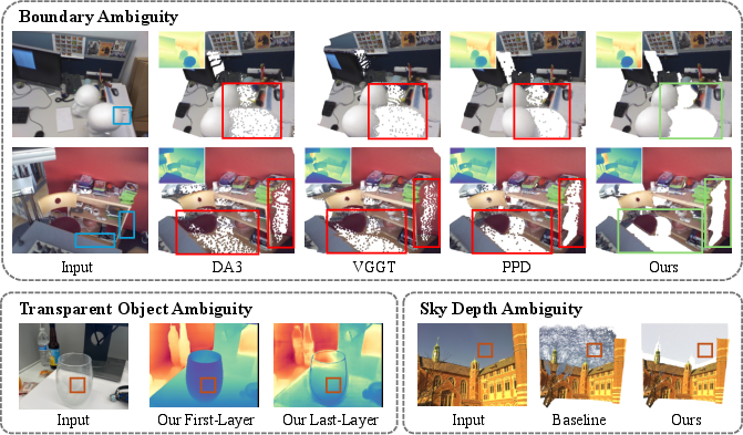
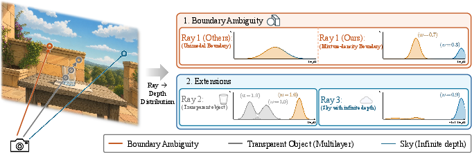
Abstract: Despite advances in depth estimation, flying points remain a persistent failure mode: near object boundaries, depth estimators often predict spurious 3D points in the empty space between foreground and background surfaces. We trace this artifact to a standard modeling choice: assigning each pixel a single depth hypothesis. At boundaries, a pixel can straddle a foreground and a background surface, so its true depth is ambiguous between the two. A model that predicts a single depth cannot keep both possibilities, so training instead pulls the prediction toward an intermediate depth that lies on neither surface. We address this with MDA, a mixture-density representation that lets the model predict multiple depth hypotheses and their associated probabilities for each pixel. Near boundaries, different hypotheses can align with different surfaces, and the decoded depth is selected from one of these hypotheses rather than placed in the empty space between them. Across different backbones, MDA substantially improves boundary reconstruction and largely removes flying-point artifacts even under severe input blur, while adding negligible runtime overhead. The same mixture-density framework naturally extends to transparent objects, where it predicts multiple depth layers at transparent pixels, and to sky regions, where a dedicated component separates the unbounded sky from finite-depth regions, producing flying-point-free skylines. Project Page: https://biansy000.github.io/mda-site/.


Paper Prompts
Sign up for free to create and run prompts on this paper using GPT-5.
Top Community Prompts
Explain it Like I'm 14
Overview
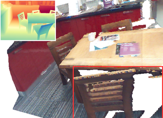
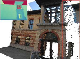
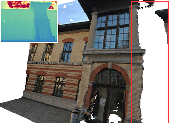
This paper tackles a common problem in computer vision called “flying points.” When computers estimate depth from images (how far each pixel is), they often make mistakes at the edges of objects. Instead of putting points on the foreground object or the background, they put “ghost” points floating in the empty space between them. The authors show why this happens and introduce a new way to predict depth that greatly reduces these floating mistakes while staying fast.
Key Questions
- Why do depth maps produce “flying points” near object boundaries?
- Can we design a model that keeps multiple valid depth choices for a single pixel instead of forcing just one?
- Will this fix work in tough cases like blurry images, transparent objects (like glass), and sky regions?
- Can we do all this without slowing the model down?
How the Method Works (in everyday language)
The problem in simple terms
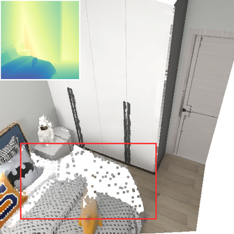
Imagine a photo of a lamp in front of a wall. At the edge of the lamp, one pixel might partly see the lamp (close) and partly see the wall (far). Most depth models are forced to pick a single number for that pixel. Because both “close” and “far” look possible, the model often picks something in between—neither on the lamp nor on the wall—creating a 3D point that floats in mid-air. That’s a flying point.
The key idea: let the model keep multiple choices
Instead of predicting one depth per pixel, the paper’s method (called MDA: Mixture-Density depth representation) predicts several depth options for each pixel and how likely each option is. Think of it like this:
- For each pixel, the model proposes K depth guesses: “it could be depth A, or depth B, or depth C…”
- It also gives a probability to each guess: “A is 70% likely, B is 25%, C is 5%,” for example.
During use, the model picks one of these guesses (not an average) to place the point on a real surface—either the foreground or the background—avoiding mid-air points.
A quick analogy for the training math
Older models acted like they were fitting a single bell curve (one “bump”) of probability around one depth value. That works on flat, unambiguous areas but fails at edges where two different depths are plausible. This paper replaces the single bell with a small “mixture” of bells—one per hypothesis—so the model can represent multiple possibilities at once. The training objective encourages the right bell to match the ground-truth depth without dragging predictions into the empty space between surfaces.
Decoding the final depth
At the end, the model selects the most likely depth hypothesis for each pixel instead of averaging them. That single choice naturally lands on a real surface and avoids flying points.
Extensions for tricky scenes
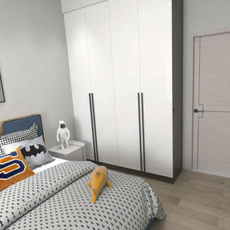
- Transparent objects (like glass): A single pixel can correspond to multiple real depths (the glass surface and the objects behind it). The method allows more than one depth to be active at once, so it can output multiple layers where needed.
- Sky: Sky is effectively “infinitely far.” The method adds a special “very far” component just for sky, so the model doesn’t place fake nearby points at the skyline.
Main Findings and Why They Matter
Here are the main results the authors report:
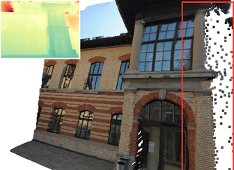
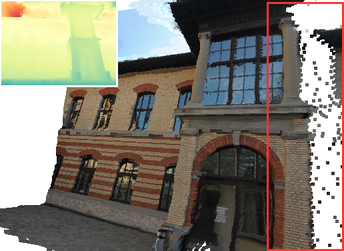
- Strongly reduces flying points at object boundaries. Compared with standard depth models and slower refinement methods, their approach creates cleaner, sharper edges where points lie on real surfaces (foreground or background), not in mid-air.
- Works even when images are blurry. When boundaries are hard to see, older methods blur and create more floating points; the mixture approach stays more stable by keeping multiple plausible depths until it can choose one.
- Fast and simple to add. It only changes the final prediction layer of existing models (like DA3 and VGGT) and adds almost no runtime cost. It’s far faster than several-step “diffusion” refiners.
- Keeps overall depth quality. On standard video depth tests, it matches or improves the base models, showing it fixes boundaries without hurting general performance.
- Handles transparent objects and sky in the same framework. It can output multiple depth layers for transparent regions and clean skylines without extra segmentation networks.
These findings matter because many 3D applications (robotics, AR/VR, 3D mapping, novel view synthesis) need accurate, clean geometry. Flying points cause collisions, visual artifacts, and planning mistakes. Reducing them improves reliability.
Implications and Impact
- For practitioners: You can upgrade existing depth models by swapping in this mixture-density head, getting cleaner boundaries with almost no speed penalty.
- For challenging scenes: The method offers a unified way to deal with depth ambiguity—edges, transparency, and sky—without special-case hacks or heavy post-processing.
- For future research: It suggests that representing uncertainty explicitly (multiple hypotheses with probabilities) beats forcing a single guess, especially where the image truly is ambiguous.
In short, by letting each pixel hold several depth possibilities and choosing wisely rather than averaging, the paper delivers flying-point-free depth maps that are sharper, more robust, and just as fast.
Knowledge Gaps
Unresolved gaps, limitations, and open questions
Below is a concise, actionable list of what remains missing, uncertain, or unexplored in the paper’s current formulation and evaluation.
- Supervision mismatch at boundaries: training still uses single-depth ground truth where multiple depths are plausible; no multi-layer supervision is available for occlusion boundaries, leaving component–surface assignment underconstrained and potentially inconsistent across scenes.
- Lack of theoretical guarantees: beyond an appendix gradient discussion, there is no formal analysis proving when the mixture likelihood avoids mid-point (flying-point) solutions or ensures component specialization to true surfaces.
- Decoding choice is heuristic: selecting the component with highest density at its mean is not justified via an optimal decision rule; comparisons to alternative decoders (e.g., MAP over continuous depth, risk-aware decoding, spatially-regularized assignments) are missing.
- Per-pixel independence: the mixture is modeled independently per pixel; there is no spatial or temporal regularization to ensure coherent surface selection across neighboring pixels or frames, risking flicker along edges in videos.
- Temporal/multi-view consistency is not studied: while video depth metrics are reported, there is no evaluation of component identity consistency across time/views, or constraints enforcing epipolar and temporal coherence of mixture assignments.
- Probability calibration is untested: mixture weights and per-component scales are treated as probabilities/uncertainties, but calibration (e.g., ECE for depth errors, reliability diagrams) is not evaluated; downstream use of these uncertainties is unexplored.
- Sensitivity to the number of components K: K is fixed (typically 4) with limited ablation; there is no study of performance vs K, diminishing returns, or adaptive/nonparametric schemes (e.g., per-pixel K or sparsity-inducing priors).
- Training stability and degeneracy: mixture MLEs can suffer component collapse or vanishing/over-confident scales; there is no quantitative analysis of failure modes, regularizers, or initialization strategies to prevent degenerate solutions.
- Limited ablations on design choices: the benefits of log-depth vs linear, Laplace vs Gaussian mixtures, mixture-weight parameterizations, and scale regularization are not systematically dissected across datasets and backbones.
- Component interpretability and permutation: although specializations are visualized, there is no metric assessing component-to-surface alignment or permutation stability across scenes/runs; mechanisms to enforce consistent roles are not explored.
- Transparent-object modeling is restricted to two layers: many real scenes exhibit more than two overlapping/translucent layers, partial transparency, or view-dependent reflections/refractions; extending beyond K=2 layers and handling refractive geometry remain open.
- Transparent classification thresholding is heuristic: the sigmoid-weight variant uses a fixed sum-of-weights threshold (1.5) to classify transparency; robustness to threshold choice and calibration on real data are not analyzed.
- Sky component is manually fixed: the sky depth mean/scale are set to large constants and not learned; the impact of these hyperparameters, their interaction with metric scale, and generalization to far-but-finite horizons are untested.
- Outdoor, in-the-wild validation is limited: evaluations are primarily on indoor/synthetic mixes; large-scale outdoor benchmarks (e.g., driving, urban panoramas) and real-world transparent/reflective scenes are underrepresented.
- Downstream 3D reconstruction is not quantified: while boundary metrics improve, the effect on full 3D pipelines (e.g., meshing quality, novel view synthesis PSNR/SSIM/LPIPS, point-cloud completeness) and on robotic grasping/planning near edges is not reported.
- Flying-point measurement is indirect: boundary CD/Acc are proxies; a direct metric that explicitly counts or distances flying points between surfaces (e.g., near-edge empty-space occupancy) is not provided.
- Computational/memory trade-offs are underreported: FPS is given, but GPU memory, training time, and scaling with K are not characterized; feasibility on resource-constrained or mobile devices is unclear.
- Robustness beyond blur: stress tests for noise, defocus, motion blur, low light, rolling shutter, compression artifacts, and lens distortion are not conducted; corresponding augmentation strategies are not explored.
- Cross-sensor generalization: behavior on different depth conventions (metric vs relative), focal ranges, fisheye/wide-FOV, and varying intrinsics/extrinsics is not systematically evaluated.
- Integration with geometry priors: the method does not exploit occlusion reasoning, layered scene models, or planar/curvature priors that could improve component assignment near edges; combining mixture density with geometric constraints remains open.
- Learning to output multiple layers at boundaries (not only transparency): the boundary variant always decodes a single layer; producing multi-layer boundary outputs (with ownership probabilities) for downstream multi-surface reconstruction is not explored.
- Using the full posterior downstream: only a single decoded depth is fed to applications; leveraging the full per-pixel mixture (e.g., for uncertainty-aware fusion, volumetric mapping, or probabilistic SLAM) is left unexplored.
- Failure-case analysis: qualitative/quantitative characterization of where the approach still produces flying points (e.g., extremely thin structures, repeated textures, heavy bloom) and why components fail to specialize is missing.
- Comparisons to alternative multi-modal approaches: beyond MoE/diffusion baselines, comparisons to cost-volume or volumetric representations that natively encode multi-hypotheses (e.g., occupancy/SDF/NeRF-style uncertainty) are absent.
Practical Applications
Overview
The paper introduces MDA, a lightweight mixture-density depth representation that replaces single-depth, unimodal predictions with multiple depth hypotheses and associated probabilities per pixel. By modeling ambiguity explicitly (e.g., foreground vs. background at occlusion boundaries), MDA markedly reduces “flying points,” improves boundary fidelity, remains robust under blur, and extends naturally to multi-layer depth for transparent objects and to threshold-free sky handling. It can be dropped into existing backbones (e.g., DA3, VGGT) with negligible runtime cost.
Below are practical applications derived from these findings, organized into immediate and long-term opportunities.
Immediate Applications
These applications can be deployed now with modest engineering effort, leveraging the paper’s mixture-density head on existing depth estimators.
- Flying-point-free 3D reconstruction and meshing
- Sectors: software, media/entertainment, AEC (architecture/engineering/construction), GIS
- What: Cleaner meshes and point clouds with sharp edges and flying-point-free boundaries from monocular or multi-view images.
- How/tools/workflows: Integrate the MDA head into DA3/VGGT within photogrammetry pipelines (e.g., RealityCapture/Metashape plug-ins, Blender add-ons) or content pipelines for 3D asset creation; use MDA’s decoded depth directly for meshing and mesh texturing.
- Dependencies/assumptions: Camera intrinsics/extrinsics for multi-view reconstruction; model fine-tuning for target domains (indoor/outdoor); K selection (e.g., K=4) and GMM variant for stability.
- AR occlusion and compositing with clean boundaries
- Sectors: mobile software, AR/VR, consumer imaging
- What: More stable and accurate real-time occlusion between virtual and real objects (e.g., fewer halos at hair, thin structures, skylines).
- How/tools/workflows: Replace phone/AR engine’s monocular depth module with MDA-enabled estimator; use the sky component for robust skyline segmentation and sky replacement; decode per-pixel depth by component selection to avoid averaged depths.
- Dependencies/assumptions: Mobile inference constraints (need a compact backbone with MDA head); domain generalization across devices and lighting; latency budget.
- Robotics navigation and manipulation with sharper geometry
- Sectors: robotics, logistics/warehousing, consumer/home robots
- What: Improved obstacle boundaries and grasp planning around thin or edge-adjacent objects (reduced false positives from flying points).
- How/tools/workflows: Swap in MDA-equipped depth in visual SLAM, voxel mapping, or grasp planners; fuse MDA depth with LiDAR or stereo for redundancy.
- Dependencies/assumptions: Robustness to motion blur and lighting (paper shows improved blur robustness); calibration and sensor fusion stack compatibility.
- Drone surveying and mapping (edge-resolved façades and skylines)
- Sectors: GIS, AEC, infrastructure inspection, surveying
- What: Cleaner building outlines, powerline edges, and skyline boundaries in photogrammetric reconstructions; fewer outlier points in clouds.
- How/tools/workflows: Incorporate MDA-based depth into aerial photogrammetry pipelines; use sky component to segment sky for better reconstruction masks and horizon detection.
- Dependencies/assumptions: Proper camera calibration; generalization to high-altitude viewpoints; wind/blur conditions (MDA is robust to blur but training on aerial data improves performance).
- Video post-production depth effects with fewer boundary artifacts
- Sectors: media/entertainment, creative tools
- What: Better rotoscoping, depth-of-field, and relighting with sharper matte boundaries and less bleeding.
- How/tools/workflows: Plug-in for NLE/compositing suites (e.g., Adobe Premiere/After Effects, DaVinci Resolve) that swaps in MDA depth; exploit per-component probabilities to refine mattes.
- Dependencies/assumptions: Runtime within editor constraints; varied content domains (film, animation, sports) may require fine-tuning.
- Sky segmentation without a separate network
- Sectors: mobile imaging, UAVs, photography apps, environmental perception
- What: Free sky masks via the dedicated sky component and cleaner skyline geometry in 3D reconstructions.
- How/tools/workflows: Use mixture weights to classify sky vs. non-sky; apply in horizon detection, sky replacement, and exposure control.
- Dependencies/assumptions: Choice of large fixed mean/scale for sky component; potential need to adjust for extreme haze or overexposure.
- Depth for neural rendering with fewer artifacts
- Sectors: software, AR/VR, graphics
- What: Provide high-quality, boundary-accurate depth priors to NeRF/3DGS pipelines, reducing floaters and speeding convergence.
- How/tools/workflows: Feed MDA depth as supervision or initialization; weight edge regions more where MDA reduces ambiguity.
- Dependencies/assumptions: Consistent scale; integration with existing training loops; domain-tuned fine-tuning recommended.
- Academic benchmarking and analysis of boundary ambiguity
- Sectors: academia, R&D
- What: A principled control for ambiguity modeling in depth estimation studies, enabling new boundary-focused benchmarks and analyses.
- How/tools/workflows: Adopt the mixture NLL and per-component visualization for analyzing dataset biases, component specialization, and boundary behavior.
- Dependencies/assumptions: Access to datasets with fine boundary ground truth (e.g., NRGBD, HiRoom); consistent evaluation protocols.
Long-Term Applications
These opportunities require additional research, scaling, training data, or systems integration beyond the current demonstrations.
- Glass-/transparency-aware robotic manipulation and bin-picking
- Sectors: robotics, manufacturing, retail/fulfillment
- What: Reliable handling of transparent and glossy items by modeling co-existing depth layers (e.g., glass and background).
- How/tools/workflows: Use the sigmoid-weighted, K=2 multi-layer extension to generate both foreground (transparent surface) and background depths; inform grasp planners and collision checking with layered geometry.
- Dependencies/assumptions: High-quality multi-layer depth datasets for training (real transparent objects); robust generalization to varied materials/lighting; sensor fusion with tactile/force feedback.
- See-through AR mapping and occlusion (glass-aware SLAM)
- Sectors: AR/VR, wearables
- What: Real-time, glass-aware mapping and occlusion in head-worn devices (e.g., mapping building interiors through windows without hallucinated surfaces).
- How/tools/workflows: Integrate multi-layer MDA into SLAM backends; maintain layered maps along rays; choose surfaces adaptively for occlusion rendering.
- Dependencies/assumptions: Real-time performance on edge devices; stability under head motion; large-scale training on transparent scenes.
- Autonomous driving and ADAS with improved occlusion handling
- Sectors: automotive
- What: Better treatment of thin structures (poles, fences, wires) and horizon/skyline boundaries; fewer false obstacles from flying points.
- How/tools/workflows: Integrate MDA as a monocular depth module within multi-sensor fusion stacks; use sky component for horizon reasoning and scene segmentation.
- Dependencies/assumptions: Extensive validation on long-tail conditions (rain, glare, night); safety certification; fusion with LiDAR/radar for redundancy.
- Digital twins and smart city models with cleaner edges
- Sectors: AEC, urban planning, infrastructure management
- What: Higher-fidelity building contours and façade details in city-scale reconstructions; reduced post-cleanup costs.
- How/tools/workflows: Embed MDA in city-scale photogrammetry workflows; impose quality gates based on boundary metrics to flag scans needing reshoot.
- Dependencies/assumptions: Scaling to massive datasets; consistent camera metadata; policy/contractual updates to accept mixture-based reconstructions.
- Consumer imaging: next-gen portrait mode and segmentation
- Sectors: consumer electronics, mobile imaging
- What: Fewer edge artifacts in synthetic bokeh and subject cutouts (e.g., around hair, glasses).
- How/tools/workflows: Deploy compact MDA models on-device; exploit component selection to avoid mid-air depth between subject and background.
- Dependencies/assumptions: Model compression/pruning; energy constraints; on-device privacy requirements.
- Standardized ambiguity-aware depth modeling in benchmarks and toolkits
- Sectors: academia, standards, policy
- What: Promote mixture-density as a default modeling choice in depth toolkits and evaluations; encourage reporting boundary-specific metrics.
- How/tools/workflows: Incorporate mixture NLL losses and decoding in common CV libraries; update benchmarks to include boundary/ambiguity splits and transparent/sky subsets.
- Dependencies/assumptions: Community adoption; availability of open-source implementations and pretrained checkpoints.
- Layered scene understanding for 3D video editing and XR telepresence
- Sectors: media/entertainment, communications
- What: Stable, layered geometry for in-the-wild video capture (fewer floaters) to enable reliable 3D edits and telepresence composites.
- How/tools/workflows: Combine MDA depth with dynamic scene models (NeRF/3DGS variants) and per-layer compositing; use sky and transparency extensions to reduce cleanup.
- Dependencies/assumptions: Real-time capture constraints; temporal consistency of component assignments; robust training on diverse scenes.
- Inspection of glass facades and powerlines with reduced false positives
- Sectors: infrastructure, energy, utilities
- What: Drones or stationary cameras capturing structures with fewer outlier points (e.g., cables, glass surfaces) for defect detection.
- How/tools/workflows: Incorporate MDA depth into inspection analytics; flag anomalies using cleaner boundary geometry and fewer floaters.
- Dependencies/assumptions: Domain-specific training (e.g., high-dynamic-range, distant thin objects); integration with existing defect detection systems.
- Extending mixture-density modeling to other ambiguous signals
- Sectors: software, research
- What: Apply mixture representations to normals, optical flow, or occupancy to capture multi-modal ambiguities (e.g., translucency, motion blur).
- How/tools/workflows: Adapt mixture NLL to other dense prediction heads; analyze component specialization; integrate into multi-task perception stacks.
- Dependencies/assumptions: Task-specific likelihoods and decoding rules; datasets with suitable supervision; careful balancing to avoid mode collapse.
Notes on feasibility across applications:
- MDA adds negligible runtime overhead when integrated as a final-layer modification, but mobile and embedded deployments require model compression and careful engineering.
- Generalization benefits from fine-tuning on target domains (indoor/outdoor, aerial, transparent objects). The multi-layer and sky variants may need additional supervision or calibrated constants.
- Component selection strategies and K values influence performance; the Gaussian-mixture variant in log-depth typically offers better stability and gradients at boundaries.
Glossary
- 3D-aware feature matching: A technique that exploits 3D geometric consistency to match features across views, improving multi-view reconstruction accuracy. Example: "with 3D-aware feature matching for better multi-view accuracy."
- Absolute Relative error (AbsRel): An evaluation metric for depth estimation that measures the mean relative error between predicted and ground-truth depths. Example: "we report Absolute Relative error (AbsRel, the mean of )"
- Argmax: The operation that selects the index of the maximum value, used here to choose the most likely mixture component at each pixel. Example: "brighter pixels indicate where head wins the argmax"
- Area averaging: A downsampling method that averages pixel values over areas to reduce resolution while preserving overall intensity. Example: "downsampling each frame by factor with area averaging and bicubic upsampling it back to the model resolution"
- Backbone: The core feature-extraction network of a model onto which task-specific heads are attached. Example: "MDA\ keeps the backbone unchanged and only modifies the final prediction layer"
- Bicubic upsampling: An image interpolation method using cubic polynomials in two dimensions to increase resolution smoothly. Example: "downsampling each frame by factor with area averaging and bicubic upsampling it back to the model resolution"
- Canny operator: A gradient-based edge detector used to identify boundaries in images or depth maps. Example: "we extract edge masks from ground-truth depth maps with Canny operator"
- Chamfer Distance (CD): A metric for comparing two point clouds by measuring average nearest-neighbor distances. Example: "We report Chamfer Distance (CD) and Accuracy (Acc; mean predicted-to-GT distance)"
- Confidence-weighted L1 loss: A regression loss where each pixel’s L1 error is scaled by a learned confidence, modeling heteroscedastic uncertainty. Example: "The network is trained to minimize confidence-weighted L1 loss over all pixels:"
- Denoising: The iterative process in diffusion models that removes noise to refine predictions. Example: "their multi-step denoising process is slow"
- Diffusion Transformer: A diffusion-based generative model architecture using transformers to progressively refine outputs. Example: "uses a pixel-space Diffusion Transformer to refine the output of feed-forward depth estimators"
- Flying points: Spurious 3D points predicted in empty space between true surfaces, typically near object boundaries. Example: "flying points, 3D points that fall in empty space between foreground and background surfaces near object boundaries"
- Gaussian Mixture Model (GMM): A probabilistic model representing data as a weighted sum of multiple Gaussian distributions. Example: "The Laplacian mixture above can be directly extended to a Gaussian Mixture Model (GMM)"
- Laplacian distribution: A probability distribution with a sharp peak and heavier tails than a Gaussian, often used with L1 losses. Example: "Assume the ground-truth depth at pixel follows a Laplacian distribution centered at the depth prediction =\alpha/ and scale $b_{\mathrm{sky}$, both set to large predefined constants"
- Softmax: A normalization function that converts logits into a probability distribution over components. Example: "The mixture weights are produced by a softmax over per-component logits."
- Threshold accuracy δ<1.25: A metric reporting the fraction of pixels whose relative error is below 1.25. Example: "and threshold accuracy (, the fraction of pixels with )"
- Unbounded sky: The conceptual modeling of sky as having infinite or extremely large depth, requiring special handling in depth estimation. Example: "a dedicated component separates the unbounded sky from finite-depth regions"
- Unimodal per-pixel representation: Modeling each pixel’s depth with a single-mode distribution, which can be too restrictive near boundaries. Example: "thereby enforcing a unimodal per-pixel representation."
Collections
Sign up for free to add this paper to one or more collections.

