Strong Stochastic Flow Maps
Abstract: Flow and diffusion models generate high-quality samples in many modalities; however, many network evaluations are required during inference due to numerical integration of an underlying differential equation. Flow maps alleviate this problem by learning the solution map of the differential equation directly, enabling few-step sampling. Yet, current methods are restricted to approximating the solution map of ODEs. These methods can be used to learn the transition kernel of an SDE, thereby obtaining a solution map that recovers the marginal distributions of the process (weak convergence) rather than the solution path (strong convergence). We propose Strong Stochastic Flow Maps (SSFMs) as a novel framework for learning the strong solution map of additive-noise SDEs, directly generalizing deterministic flow maps to the stochastic setting. Further, a polynomial approximation to Brownian motion is introduced and shown to converge pathwise. These results enable a simulation-free training objective for the solution map of diffusion models. We demonstrate that SSFMs outperform previous stochastic flow map methods on image generation and enable few-step sampling of molecular systems.

Paper Prompts
Sign up for free to create and run prompts on this paper using GPT-5.
Top Community Prompts
Explain it Like I'm 14
What this paper is about (big picture)
This paper is about making fast and accurate “generators” that create things like images or molecule shapes using math models that include randomness. Today’s best generators (diffusion and flow models) usually need lots of tiny steps to work well, which is slow. The authors introduce Strong Stochastic Flow Maps (SSFMs), a new way to jump in just a few steps while still following the random “wiggles” of the process. This makes generation much faster without losing accuracy.
What the researchers wanted to figure out
They set out to do four things, in plain terms:
- Learn to predict not just “snapshots” of where a system ends up, but the actual random path it takes (like watching a whole movie, not just flipping through photos).
- Do this for systems with randomness (SDEs), not only for deterministic systems (ODEs).
- Find a compact, easy-to-handle way to feed “what the randomness did” into a neural network.
- Train the model without slow, heavy simulations, and show it works on images and molecules in just a few steps.
How they approached it (with simple analogies)
Think of moving from time s to time t as traveling from one place to another:
- In a normal flow map (deterministic), you follow a fixed set of directions.
- In a stochastic setting (with randomness), wind gusts push you around as you walk.
The authors’ key ideas:
- The Itô map: This is like a “super-GPS” that, given your start point and a specific pattern of wind gusts, tells you exactly where you’ll end up. SSFMs try to learn this map directly.
- Strong vs. weak solutions:
- Weak (older methods): Match the distribution of where travelers end up at each time, but not the exact path each traveler took. It’s like making sure the crowd gathers in the right places without tracking individual routes.
- Strong (this paper): Match what happens to each individual path when the same wind gusts occur. Same wind pattern → same path → same destination, no matter how many steps you take. It’s like replaying the exact journey with the same random pushes.
How they make randomness easy to use:
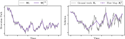
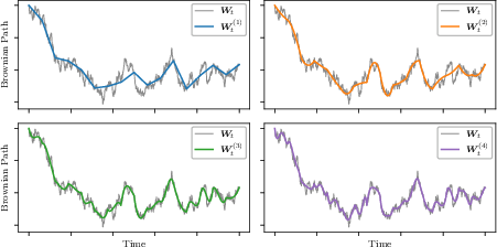
- Brownian motion is the math model for “random wiggles” (the wind gusts). It’s a squiggly line that’s hard to feed into a network directly.
- The trick: summarize that squiggly line with just a few numbers using a polynomial expansion (built from Legendre polynomials). Think of it as capturing the main bends and wiggles of a line with a short list of coefficients.
- These coefficients are:
- Easy to sample (they’re independent and normally distributed).
- Guaranteed to approximate the true random path better as you include more of them.
- Easy to “stitch together” for consecutive time segments (so two short trips combine into one longer trip smoothly).
How they train SSFMs:
- They design a neural “jump” from time s to t that depends on:
- The current state,
- The compact “wind summary” (those coefficients),
- And a form like a one-step Euler–Maruyama update (a standard recipe for stepping through random systems).
- Two-part self-distillation loss: 1) Local matching: For very small jumps, the model’s behavior must match the known small-step behavior of the true system (so it learns the right “instant direction and randomness”). 2) Semigroup (consistency) loss: Going from s→u→t should match going s→t in one go (like two short hops equal one long hop). This enforces path consistency.
- For diffusion models (used in image generation), they can build this training objective without running slow long simulations by using known formulas for the reverse process. That makes training more efficient.
What they found and why it matters
- Better accuracy with fewer steps:
- On image datasets (CIFAR-10 and CelebA-64), SSFMs beat earlier stochastic flow maps and are competitive with top deterministic shortcut methods, even with very few steps (like 2–16).
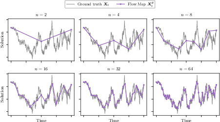
- They showed a “strong” property: if you start with the same noise and use the exact same randomness, you get the same final image, regardless of whether you take 2, 4, 8, or 16 steps. That means the model truly understands the path, not just the end result.
- Compact randomness works:
- Using just a small number of polynomial coefficients to summarize the random path is enough for accurate results, and adding more coefficients improves accuracy in a predictable way.
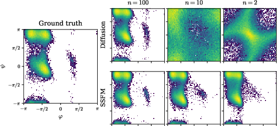
- Molecular generation:
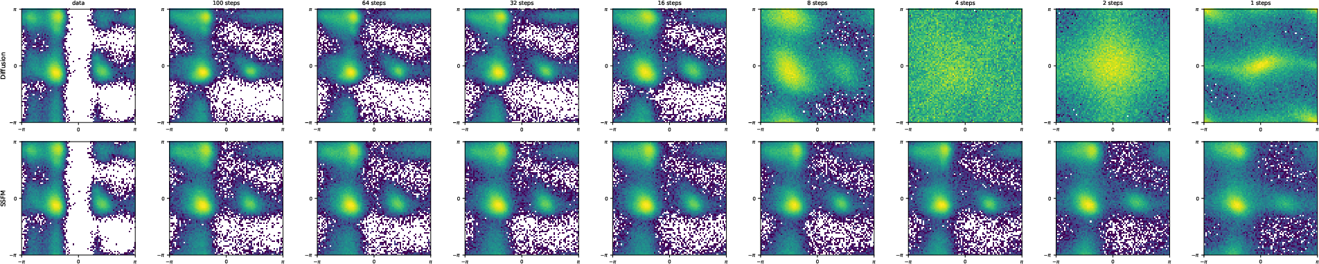
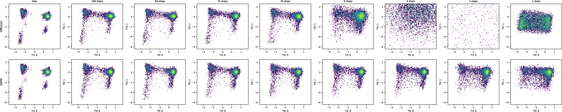
- On molecules (Alanine Dipeptide and Chignolin), SSFMs produce accurate samples with as few as 1–4 steps, and match the quality of much slower many-step diffusion baselines. This is important for scientific simulations where speed matters a lot.
Why this is important:
- Fewer steps mean faster generation at test time (less waiting, less compute).
- Strong, pathwise modeling allows you to measure “along-the-way” quantities (pathwise observables), not just final outcomes. That’s useful in science and engineering.
What this could change going forward
- Faster, more reliable generators: SSFMs can make high-quality images and molecular structures quickly, which could help creative tools and scientific research.
- Better physics-aware models: Because SSFMs keep paths consistent, they’re well-suited for tasks that depend on the entire trajectory, not just the endpoint (like measuring energy along a reaction path).
- Broader impact: The approach could help align generative models with path-based rewards, speed up molecular simulations, and inspire new methods in any domain where randomness matters.
Overall, the paper shows how to learn “the whole movie” of a random process in a compact, fast way—and that doing so pays off in practice.
Knowledge Gaps
Below is a consolidated list of concrete knowledge gaps, limitations, and open questions that remain unresolved by the paper. Each point is framed to help guide future research directions.
- Extension beyond additive noise: The method and theory target additive-noise SDEs; it is unclear how to extend SSFMs to multiplicative/state-dependent diffusion where the Itô map is discontinuous and rough-path machinery (and Lévy areas) is required.
- Higher-order stochastic structure: For multiplicative noise, the approach would need iterated integrals (e.g., Lévy area) in addition to Brownian increments; how to design a tractable coefficient representation and training objective in that setting is open.
- Quantitative error bounds at finite N: While convergence is established as polynomial degree , explicit finite- error rates (in -Hölder and strong pathwise metrics) are not provided, nor criteria to choose adaptively per step size.
- Step-size versus degree trade-off: There is no principled schedule tying time step size and polynomial degree to guarantee a target strong error; adaptive control strategies are unstudied.
- Scalability of Brownian input: For high-dimensional states (e.g., images, molecular coordinates), passing of dimension equal to the Brownian dimension may be prohibitive; the paper does not specify how the Brownian coefficients are represented, compressed, or embedded at scale.
- Choice of Brownian dimension: It is unclear how the Brownian dimensionality is selected in practice for image models (per-pixel, per-channel, latent space?), and how this choice affects fidelity, diversity, and computational cost.
- Numerical stability of Chen relations: Although closed-form Chen relations are claimed, the paper does not assess their numerical stability or error accumulation when chaining many intervals in high dimensions.
- Objective sufficiency and identifiability: The self-distillation loss enforces two-segment semigroup consistency only; it is unknown whether this is sufficient for global semigroup consistency across longer chains, or whether additional constraints are needed to avoid degenerate solutions.
- Choice of midpoint u and schedule: The distillation uses ; the impact of different split strategies or multi-segment consistency (beyond two segments) on accuracy and stability is not explored.
- Learning vs fixing diffusion g(t): For diffusion models, is known; the benefits/risks of learning $\bg^\theta_{s,t}$ versus fixing it (and implications for bias and stability) are not ablated.
- Dependence on teacher signals: The “simulation-free” training still requires access to ground-truth drift (e.g., reverse-time drift from a score model); the dependence on pre-trained scores, their accuracy, and error propagation to SSFMs are not quantified.
- Generality beyond diffusion SDEs: Outside diffusion modeling (where drift is specified via known objectives), how to train SSFMs when only samples from the terminal distribution are available and no simulator/score oracle exists remains open.
- Theoretical optimization guarantees: The uniqueness-of-minimizer result is asymptotic/idealized; convergence guarantees under finite data, nonconvex optimization, and finite-capacity networks (and potential failure modes) are not provided.
- Robustness to inference step count: Although pathwise consistency is illustrated, the degradation in sample quality as a function of NFE (especially at 1–2 steps) is not systematically analyzed or bounded.
- Comparison breadth: Empirical comparisons omit strong modern ODE/SDE samplers (e.g., high-order DPM solvers) and larger benchmarks (e.g., ImageNet, class-conditional tasks), limiting conclusions about competitiveness at scale.
- Guidance and conditioning: How SSFMs interact with classifier-free guidance, conditioning signals, and control inputs (text, class, guidance strength) is not explored.
- Pathwise observable estimation: Despite promising claims, there are no experiments demonstrating estimation of pathwise observables (e.g., time correlations, first-passage times) and how SSFMs compare to standard SDE integrators for these tasks.
- Physical constraints in molecular systems: Whether SSFM-generated trajectories preserve detailed balance, ergodicity, or other thermodynamic/physical constraints at few steps is unverified; long-time kinetic properties are not evaluated.
- Coverage vs fidelity trade-offs: The impact of injecting Brownian randomness via SSFMs on diversity/mode coverage (versus deterministic flow maps) is not analyzed beyond FID.
- Hyperparameter sensitivity: The effects of key training hyperparameters (polynomial degree N, Δt threshold, split η, EMA decay β) on accuracy, stability, and strong error are not ablated.
- Computational profile: There is no analysis of training/inference wall-clock time, memory, and throughput versus baselines, including overhead from generating and manipulating polynomial coefficients and Chen compositions.
- Architectural choices: The rationale for separate networks for and , potential sharing, and architecture ablations (e.g., alternative backbones) are not investigated.
- Time reparameterization: Sensitivity to different noise schedules/time warps and whether certain schedules improve strong approximation quality or reduce required N is not explored.
- Alternative bases: Only shifted Legendre polynomials are considered; whether other bases (Fourier, wavelets, learned bases) yield better approximation/Chen properties or improved stability remains an open design choice.
- Multi-resolution path features: Combining coarse and fine polynomial coefficients adaptively across time (or using hierarchical bases) to improve accuracy at fixed N is unstudied.
- Multi-step training curricula: Training with longer semigroup chains (3+ segments) or curriculum strategies for consistency is not explored and may further improve global pathwise correctness.
- Uncertainty calibration: Whether SSFMs provide calibrated uncertainty over trajectories (and how to assess or improve calibration) is not addressed.
- Failure analyses: Cases where SSFMs underperform deterministic flow maps (e.g., certain CelebA-64 settings) are not analyzed to diagnose when stochastic pathwise modeling helps or hurts.
- Reproducibility details: Some implementation specifics (exact coefficient formulas used in code, embedding of Brownian coefficients, dimension choices, and numerical safeguards) are not fully documented, limiting reproducibility and adoption.
Practical Applications
Immediate Applications
The following applications can be deployed now by integrating SSFMs into existing diffusion/SDE-based workflows, leveraging the paper’s simulation-free training objective, few-step sampling, and pathwise (strong) convergence.
- Image generation at low latency and cost
- Sectors: software, creative media, advertising, e-commerce
- What it looks like: An “SSFM sampler” module for existing diffusion pipelines (e.g., Stable Diffusion/EDM-style backends) that delivers comparable FID with 2–8 NFEs; step-agnostic reproducibility (same Brownian path → same output) across different step counts for A/B tests and content pipelines.
- Tools/workflows: PyTorch/JAX inference layer that replaces multi-step samplers; seedable “noise keys” (polynomial Brownian coefficients) stored alongside prompts for exact reruns.
- Assumptions/dependencies: Reverse SDE/flow field available from a trained diffusion/flow-matching model; additive-noise assumption; polynomial degree N≈2–4 suffices; minor re-training for SSFM objective.
- On-device and edge generative AI
- Sectors: mobile, AR/VR, gaming, embedded systems
- What it looks like: Few-step SSFM models deployed on phones/AR glasses for real-time image edits or style transfer with strict energy/latency budgets.
- Tools/workflows: Quantization-aware training of the SSFM heads (f,g), caching Brownian coefficients as compact “noise keys.”
- Assumptions/dependencies: Model compression and memory fit on-device; additive-noise diffusion backbones; thermal/power constraints.
- Reproducible stochasticity for audits and experiments
- Sectors: software quality, trust & safety, MLOps, regulated industries
- What it looks like: “Path-consistent randomness” where the same Brownian coefficients yield identical outputs irrespective of step count, enabling defensible A/B testing, audit trails, and consistent creative iterations.
- Tools/workflows: Versioned “noise key” artifacts; pipeline hooks that propagate Brownian polynomial coefficients and apply Chen relations to compose sub-steps.
- Assumptions/dependencies: Organization-wide RNG standards; secure storage of noise keys (privacy/compliance considerations).
- Rapid molecular conformation generation
- Sectors: pharmaceuticals, biotechnology, cheminformatics
- What it looks like: 1–4 NFE SSFM generators producing equilibrium-like conformer ensembles (e.g., alanine dipeptide, small peptides) for docking, MD warm starts, and screening.
- Tools/workflows: RDKit/OpenMM plugins that call SSFM to sample conformers; batch inference to generate ensembles per molecule.
- Assumptions/dependencies: Training data for target equilibrium distributions; additive-noise SDEs for the system; validation against PMF/JS metrics.
- Accelerated Boltzmann sampling for materials screening
- Sectors: materials science, energy, catalysis
- What it looks like: Few-step SSFM surrogates approximating equilibrium distributions for candidate materials to prune design space before expensive simulations.
- Tools/workflows: Integration into high-throughput screening pipelines, scoring and ranking via pathwise observables computable from SSFM.
- Assumptions/dependencies: Reliable mapping from the design’s energy landscape to an additive-noise SDE; out-of-distribution behavior monitored.
- Pathwise reward alignment and variance reduction
- Sectors: foundation models, applied ML research
- What it looks like: Using SSFM’s pathwise consistency to compute and optimize pathwise observables (e.g., differentiable reward terms) for alignment and reinforcement learning.
- Tools/workflows: Training loops that backpropagate through SSFM outputs; plug-in loss terms for pathwise rewards or constraints.
- Assumptions/dependencies: Differentiable pipelines; well-specified reward signals; stability of self-distillation objective.
- Time-series imputation and scenario generation
- Sectors: healthcare (vitals), manufacturing (sensor data), IoT
- What it looks like: Additive Neural SDE models distilled into SSFMs for rapid, step-agnostic sampling of future trajectories with reproducible stochasticity (scenario analysis, imputation).
- Tools/workflows: SSFM heads for learned additive-noise SDEs; library utilities to carry noise keys across forecast horizons.
- Assumptions/dependencies: Valid additive-noise SDE fit to data; careful calibration; handling non-stationarity.
- Training-time acceleration via simulation-free self-distillation
- Sectors: ML infrastructure, research labs, startups
- What it looks like: Replacing long-rollout training with the SSFM self-distillation objective to reduce training cost of new few-step samplers for existing diffusion backbones.
- Tools/workflows: MLOps recipes for two-head networks (f,g), EMA teacher-student distillation, and polynomial Brownian sampling.
- Assumptions/dependencies: Access to conditional scores/flow fields; stable tuning of Δt, EMA decay, and N; adequate compute for initial teacher model.
Long-Term Applications
The following applications require further research or engineering—primarily to extend beyond additive noise, scale to complex domains, or meet regulatory and safety requirements.
- Strong flow maps for multiplicative-noise SDEs
- Sectors: finance (stochastic volatility), neuroscience, climatology
- What it could be: Rough-path/Itô–Lyons generalization of SSFM to state-dependent diffusion, enabling pathwise strong surrogates for widely used SDEs.
- Dependencies: Theoretical advances for robust training; stable parameterizations of state-dependent diffusion; benchmarks across domains.
- Real-time generative video/audio with controllable stochasticity
- Sectors: media, gaming, telepresence
- What it could be: SSFM-based video/audio diffusion achieving interactive rates (few NFEs/frame) with consistent “noise keys” for edits and collaboration.
- Dependencies: Scalable architectures, streaming training data, memory-efficient conditioning; fast I/O and on-device acceleration.
- Stochastic control and planning in robotics
- Sectors: robotics, autonomy, logistics
- What it could be: SSFM surrogates for uncertain dynamics enabling fast, consistent rollouts in MPC/planning, safety verification, and robustness testing.
- Dependencies: Valid SDE models of robot/environment noise; tight integration with control stacks; closed-loop validation.
- Uncertainty-aware digital twins
- Sectors: energy, manufacturing, process industries
- What it could be: Few-step, pathwise-consistent simulators for rapid what-if analysis with consistent uncertainty propagation across temporal resolutions.
- Dependencies: Identification and validation of plant-level SDEs; data pipelines and governance for twin updates; tooling for scenario management.
- Financial risk and stress testing
- Sectors: finance, insurance
- What it could be: Path-consistent scenario generators (MC) for portfolio/risk engines with fewer steps and reproducibility across discretizations.
- Dependencies: Extension to multiplicative noise and jumps; regulatory model risk approval; robust calibration and backtesting.
- Surrogates for stochastic PDEs and climate/CFD subgrid models
- Sectors: climate, aerospace, automotive
- What it could be: Learning strong solution maps for latent SDE components or SPDE-inspired surrogates (e.g., turbulence closures), enabling faster ensembles.
- Dependencies: Methodological extensions from SDEs to SPDEs; stability and conservation constraints; large-scale training data.
- Personalized healthcare trajectory simulation
- Sectors: healthcare, digital health, policy evaluation
- What it could be: Patient-level SDE models distilled into SSFMs for counterfactual policy testing with pathwise metrics (e.g., dosing strategies).
- Dependencies: High-quality longitudinal data; bias/fairness evaluation; clinical validation and governance.
- Standards and education for reproducible generative stochasticity
- Sectors: policy, standards bodies, education
- What it could be: “Noise key” standards for reproducibility/auditing in generative systems; teaching toolkits illustrating strong vs. weak convergence in SDEs.
- Dependencies: Community and regulator buy-in; privacy/security guidance for storing and sharing randomness keys; curricular development.
Notes on Feasibility and Cross-Cutting Dependencies
- Additive-noise assumption: Current SSFM theory and empirical results target additive-noise SDEs with known diffusion g(t); adoption beyond this requires research.
- Brownian polynomial approximation: Finite-degree N trades accuracy vs. compute; N≈3–4 worked in experiments but domain-specific tuning is needed.
- Training signals: Simulation-free training assumes access to conditional scores/flow-matching fields or ground-truth drift/diffusion; otherwise, simulation-based supervision is required.
- Reproducibility and security: “Noise keys” enable audits but introduce data management and privacy considerations; secure, versioned storage is advised.
- Generalization: Image and small-molecule benchmarks demonstrate feasibility; scaling to large, heterogeneous systems (e.g., proteins, climate) will need domain-specific modeling and validation.
- Tooling: Widespread adoption benefits from reference implementations in major frameworks, exportable to mobile/edge (e.g., ONNX, Core ML), and clean APIs for noise key handling.
Glossary
- Additive-noise SDEs: Stochastic differential equations where the diffusion term does not depend on the state, i.e., noise is added independently of the state. "additive-noise SDEs"
- Affine Gaussian probability paths: Interpolations between source and target distributions where intermediate marginals are Gaussian with affine dependence on endpoints. "affine Gaussian probability paths"
- Boltzmann sampling: Drawing samples from Boltzmann (Gibbs) distributions, often for molecular systems or energy-based models. "Boltzmann sampling"
- Brownian motion: A continuous-time stochastic process with independent, normally distributed increments, serving as the driving noise in SDEs. "standard Brownian motion"
- Chen relations: Algebraic rules that describe how path integrals over adjacent intervals compose, central in rough paths and signatures. "closed form Chen relations"
- Consistency models: Flow-map-like generative models trained to produce consistent multi-step outputs across discretizations. "consistency models"
- Diffusion coefficient: The (often time-dependent) matrix scaling the Brownian increments in an SDE. "diffusion coefficient"
- Drift coefficient: The deterministic vector field governing the mean dynamics in an SDE. "drift coefficient"
- Euler–Maruyama: A first-order numerical scheme (and here, parameterization) for SDEs that discretizes drift and diffusion with Brownian increments. "Euler-Maruyama parameterization"
- Fokker–Planck: The partial differential equation describing the time evolution of the probability density of a diffusion process. "Fokker-Planck"
- Flow matching: A training framework that learns a time-dependent vector field so that integrating it transports a source distribution to a target distribution. "flow matching"
- Flow map: The solution operator that maps an initial state (and possibly a driving path) to the state at a later time. "Flow maps alleviate this problem"
- GLASS flows: A class of stochastic flow-map baselines that learn transition behavior for generative modeling. "GLASS flows"
- Hölder distance: A metric assessing closeness of functions/paths based on Hölder continuity with exponent α. "-H\"older distance"
- Itô map: The pathwise solution map that takes an initial condition and a Brownian path segment to the SDE solution at a later time. "It^o map"
- Itô SDE: An SDE interpreted in the Itô sense, where stochastic integrals are adapted and have martingale properties. "It^o SDE"
- Itô–Lyons map: The extension of the Itô map in rough path theory that yields a continuous solution map for SDEs with rough signals. "It^o-Lyons map"
- Jensen–Shannon (JS) divergence: A symmetric measure of dissimilarity between probability distributions. "JS divergence"
- Legendre polynomials (shifted): Orthogonal polynomials on [0,1] used here to build a polynomial basis for Brownian motion increments. "shifted Legendre polynomials"
- Marginal vector field: The time-dependent field whose flow matches the current marginal distribution of the interpolating process. "marginal vector field"
- Neural differential equations: Models that represent vector fields (for ODEs/SDEs) with neural networks and integrate them to define transformations. "neural differential equations"
- Neural SDEs: Stochastic differential equations whose drift and/or diffusion terms are parameterized by neural networks. "Neural SDEs"
- Number of Function Evaluations (NFEs): The count of times a neural vector field is evaluated during numerical integration or sampling. "number of function evaluations (NFEs)"
- Pathwise observables: Quantities depending on entire trajectories (paths) rather than only marginal distributions at fixed times. "pathwise observables"
- Polynomial approximation of Brownian motion: Representing Brownian paths on an interval using a finite set of polynomial basis coefficients for efficient conditioning. "polynomial approximation of the Brownian motion"
- Probability flow ODE: The deterministic ODE whose solution has the same marginals as a given diffusion process. "probability flow ODE"
- Potential of Mean Force (PMF): An effective free-energy landscape over selected coordinates, often evaluated via squared error metrics in molecular tasks. "PMF squared error"
- Ramachandran plots: Density plots of protein backbone dihedral angles (ϕ, ψ) used to assess conformational sampling quality. "Ramachandran plots"
- Rough path theory: A framework extending stochastic calculus by enhancing paths with iterated integrals to ensure continuity of solution maps. "rough path theory"
- Score matching: A training objective that learns the score (gradient of log-density) to enable diffusion model inference. "score matching"
- Self-distillation: A training strategy where a model enforces consistency of its own multi-step predictions across different discretizations. "self-distillation"
- Semigroup condition: The compositional property that the flow from s to t equals the composition of flows from s to u and u to t. "semigroup condition"
- Stochastic Taylor expansion: An expansion of SDE solutions in terms of iterated stochastic integrals (e.g., of Brownian motion). "stochastic Taylor expansion"
- Strong convergence: Convergence of approximate solutions to match sample paths (not just distributions) of the target process. "strong (convergence in path)"
- Strong Stochastic Flow Maps (SSFMs): The proposed framework that learns the pathwise solution map of additive-noise SDEs given Brownian inputs. "Strong Stochastic Flow Maps (SSFMs)"
- tICA projection: Time-lagged independent component analysis projection used to assess dynamic modes of molecular systems. "tICA projection"
- Tangent condition: The requirement that an infinitesimal step of the learned flow matches the SDE’s drift and diffusion at the diagonal (s=t). "tangent condition"
- Transition kernel: The conditional distribution p(X_t | X_s) that governs transitions of a Markov process between times s and t. "transition kernel"
- Variance preserving diffusion SDE: A diffusion process whose forward (and reverse-time) dynamics maintain a controlled variance schedule. "variance preserving diffusion SDE"
- Wasserstein distance: An optimal-transport metric between probability distributions, used here for evaluation in projected spaces. "Wasserstein metrics"
- Weak convergence: Convergence in distribution of processes or approximations, without requiring pathwise agreement. "weak (convergence in distribution)"
- Weak stochastic flow maps: Flow-map approaches that target transition distributions rather than pathwise solutions of the underlying SDE. "Weak stochastic flow maps."
Collections
Sign up for free to add this paper to one or more collections.

