Information-geometric adaptive sampling for graph diffusion
Abstract: Standard diffusion models for graph generation typically rely on uniform time-stepping, an approach that overlooks the non-homogeneous dynamics of distributional evolution on complex manifolds. In this paper, we present an information-geometric framework that reinterprets the diffusion sampling trajectory as a parametric curve on a Riemannian manifold. Our key observation is that the Fisher-Rao metric provides a principled measure of the intrinsic distance. By analyzing this metric, we derive the Drift Variation Score (DVS), a geometry-aware indicator that quantifies the instantaneous rate of distributional change. Unlike prior heuristic-based adaptive samplers, our DVS solver enforces a constant informational speed on the statistical manifold, automatically maintaining a uniform rate of distributional change along the sampling trajectory. This equal arc-length strategy ensures that each discretization step contributes equally to the information speed. Theoretical analysis verifies that DVS characterizes the local stiffness of the sampling dynamics in the Fisher-Rao sense. Experimental results on molecule and social network generation show that DVS significantly improves structural fidelity and sampling efficiency. Code is at https://github.com/kunzhan/DVS
Paper Prompts
Sign up for free to create and run prompts on this paper using GPT-5.
Top Community Prompts
Explain it Like I'm 14
Easy-to-Understand Summary of “Information-Geometric Adaptive Sampling for Graph Diffusion”
What this paper is about
This paper is about teaching computers to create realistic graphs, like molecules or social networks, using a method called diffusion models. The authors introduce a smarter way to choose how big each step should be when the computer generates these graphs. Their idea, called DVS (Drift Variation Score), helps the model take small steps when things are changing fast and big steps when things are calm—so it’s both accurate and efficient.
What questions the paper asks
The researchers focus on simple, practical questions:
- Can we make graph generation more accurate by taking different-sized steps instead of always using the same step size?
- Can we automatically figure out when to slow down or speed up during generation based on how quickly the “shape” of the data is changing?
- Can we do this without retraining the model and without guessing a fixed schedule?
How the method works (with simple analogies)
Think of generating a graph as going on a hike across a landscape:
- Traditional methods walk forward using the same-sized steps, no matter if the ground is flat or rocky. That can waste time on flat parts and cause stumbles on rocky parts.
- The authors’ method uses a kind of “smart pedometer” that senses how quickly the surroundings are changing—not in physical space, but in “information space.” When the path gets twisty or steep (changes happen fast), it takes smaller steps. When it’s straight and smooth (changes are slow), it takes bigger steps.
Key ideas explained simply:
- Graphs: Think of nodes (dots) connected by edges (lines). Molecules are graphs where atoms are dots and bonds are lines.
- Diffusion model: Starts from random noise and gradually shapes it into a realistic graph by repeatedly updating it.
- Step size: How far forward the model moves at each update.
- Information distance: A way to measure how much the model’s prediction “really changes” from one step to the next—not just in numbers, but in what those numbers mean.
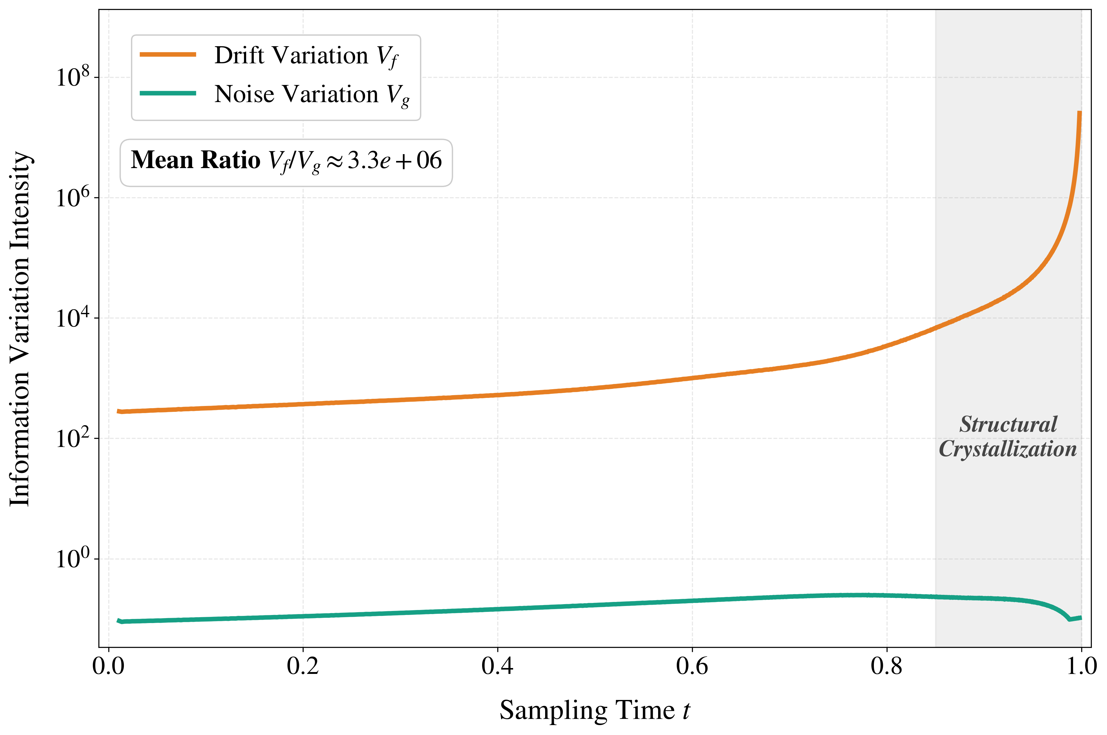
- DVS (Drift Variation Score): A number that tells you how fast things are changing right now. If DVS is high, the model should slow down (small step). If DVS is low, it can speed up (big step).
What’s new:
- The authors view the whole sampling process as moving along a curved surface called a “statistical manifold” (think of a gently curved map of possibilities).
- They use a standard tool from statistics called the Fisher-Rao metric to measure true “information distance” on that surface.
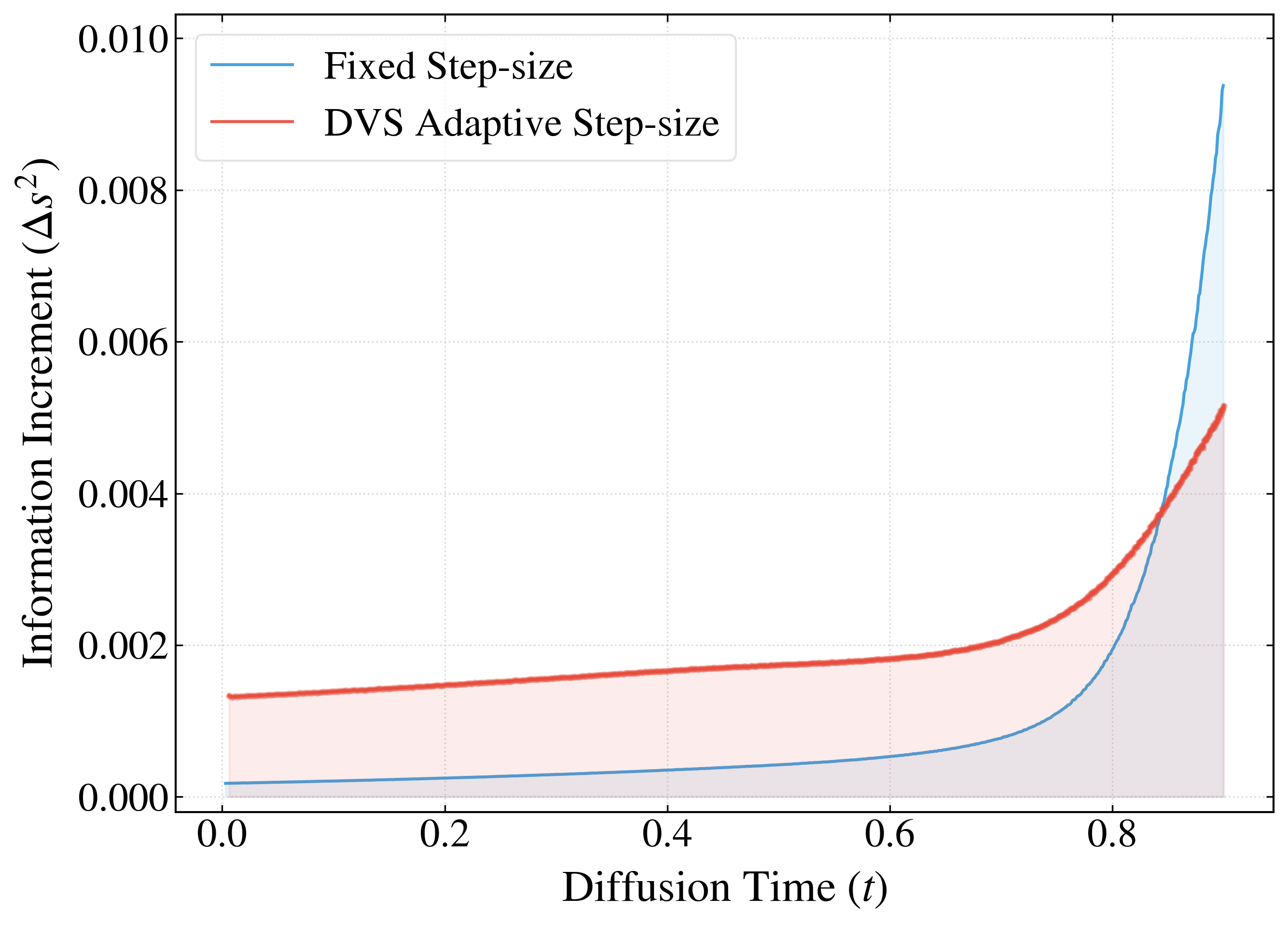
- From this, they build DVS, which measures how much the model’s direction is changing relative to noise. The sampler adjusts step size so every step covers about the same amount of information change—like taking equal-length strides in “information space.”
How it’s implemented for graphs:
- Graphs have both node features (what each dot is like) and edges (which dots are connected). These can change at different speeds.
- The method computes separate DVS values for nodes and edges, smooths them to avoid being fooled by random noise, and then picks the final step size based on whichever one needs the smaller, safer step. This keeps the whole graph stable.
What the experiments show and why it matters
The authors test their approach on:
- Molecule datasets (QM9, ZINC250k)
- General graph datasets (like synthetic and social networks)
Main takeaways:
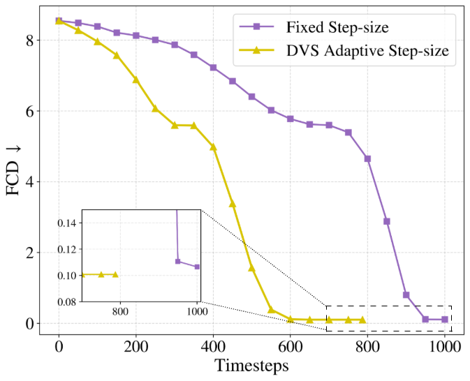
- Better quality: The generated graphs match real graphs more closely across several metrics (like FCD for molecules and MMD-based measures for general graphs).
- More stable: The sampler avoids the “rushing” that often causes errors near the end of generation, when fine details (like chemical bonds) matter most.
- More efficient: It often finishes in fewer steps than the usual methods, saving time without sacrificing quality.
- Strong even with simple solvers: Their adaptive stepping (DVS-Euler) can rival or beat more advanced non-adaptive methods (like fixed-step Heun), showing that placing steps smartly can matter more than using a fancier solver.
Why this is important:
- For molecule generation, accuracy in the final, low-noise phase is crucial to getting valid chemical structures. DVS helps the model focus its effort there.
- For social networks and other graphs, it preserves key structures better—like communities and patterns—by adapting during sensitive phases.
What this could lead to in the future
- Plug-and-play: This method doesn’t need retraining and can be dropped into existing diffusion models to improve them.
- Faster design: In drug discovery, better and faster molecule generation could speed up finding promising candidates.
- Broader use: The idea of “equal information per step” could help in other areas, like 3D shapes or scenes, where different parts change at different speeds.
- More trustworthy generation: By paying attention to where the model struggles, the method can reduce errors and make results more reliable.
In short, the paper proposes a simple but powerful idea: instead of counting time equally between steps, count “information change” equally. That makes the model spend effort where it matters most, leading to better and faster graph generation.
Knowledge Gaps
Knowledge gaps, limitations, and open questions
The paper introduces a Fisher–Rao-motivated Drift Variation Score (DVS) for adaptive time-stepping in graph diffusion. The following unresolved issues identify what is missing, uncertain, or left unexplored, and suggest concrete avenues for future work:
- Assumption on diffusion scale: The derivation treats the noise scale as locally constant and isotropic. How does DVS generalize when is strongly time-/state-dependent or anisotropic (e.g., dimension-wise or component-wise covariance), and what is the correct Fisher–Rao metric in those cases?
- Transition-kernel modeling for discrete structures: The method relies on a Gaussian transition kernel to derive the Fisher–Rao metric, yet graph edges are often modeled as discrete/categorical variables. How to derive and implement DVS for non-Gaussian (e.g., Bernoulli/Categorical/Gumbel-Softmax) transitions, and does the equal-arc-length principle still hold?
- OU/Schrödinger bridges: Exact OU-bridge transitions have time-dependent mean reversion and covariance. Can the Fisher–Rao line element and DVS be re-derived for the exact OU-bridge kernel, and does it change the adaptive rule or performance near endpoints?
- Theoretical error guarantees: There is no proof that enforcing approximately constant Fisher–Rao “informational speed” minimizes (or evenly distributes) numerical error for Euler/Heun or improves weak/strong convergence for SDEs. Can one bound local/global discretization error (or sample-quality degradation) as a function of and the chosen step-size control?
- Relation to stiffness and stability: The claim that DVS measures “local stiffness in the Fisher–Rao sense” lacks a formal stability analysis. Under what conditions does controlling guarantee stability for stiff regimes, and how does this compare to classical adaptive-step stability theory?
- Hyperparameter dependence: Key controller hyperparameters (, , , , , base step) are fixed heuristically, with limited ablation (only ). How can these be selected automatically (e.g., to hit a target NFE or error tolerance), and how sensitive is performance across datasets and models?
- Constant-arc-length target selection: The method does not specify how to set the desired (approximate) constant or its relation to target computational budget and accuracy. Can a principled controller connect “information distance per step” to NFE or error bounds?
- End-of-trajectory stiffness: The method often reaches near the data regime, limiting compensation for curvature. Can event detection, dynamic regridding, or adaptive tightening of mitigate the late-stage spike without excessive NFEs?
- Multi-component coupling design: The node/edge coupling takes the minimum of component-wise steps and replaces both EMA states by , which collapses modality-specific information. Is there a principled vector-valued controller (e.g., weighted combination, per-component subcycling, or constrained multi-objective control) that avoids bottlenecking and preserves distinct dynamics?
- Scale invariance with graph size: uses an norm that scales with dimensionality. How to normalize DVS to be invariant to graph size (number of nodes/edges) and feature scaling so that larger graphs are not unfairly forced into tiny steps?
- Robustness to score noise: Finite-difference drift estimates and single-path DVS can be noisy, especially in high-noise regimes. Would trajectory ensembles, mini-batched DVS, or uncertainty-aware smoothing (beyond fixed ) improve reliability and reduce missteps?
- Predictor–corrector integration: The paper does not specify how DVS interacts with corrector (Langevin) steps. Can DVS adapt both predictor and corrector step sizes and counts, and how does this affect training-time/test-time noise alignment?
- Solver generality: Experiments cover Euler and Heun only. How does DVS integrate with higher-order/modern solvers (e.g., DPM-Solver, RK45, PLMS/iPNDM variants, implicit/BDF methods) and does it still confer benefits?
- Comparison to adaptive controllers: There is no empirical comparison to classical adaptive step-size controllers (embedded RK, PI controllers) or recent adaptive schedules (e.g., AYS/JYS) under equal NFE or wall-clock constraints. How does DVS fare against these baselines?
- Automatic activation intervals: On some datasets the method applies DVS only in hand-picked time intervals. Can the activation be made self-triggered using thresholds or other criteria, removing manual selection?
- Preservation of bridge endpoint constraints: For OU/SB bridges, does the adaptive time grid preserve the exact endpoint constraints and marginals, and are there conditions on the time sequence that guarantee this?
- Impact on diversity and mode coverage: Larger steps in “stable” regimes might skip subtle modes. How does DVS affect diversity, novelty, and mode coverage in graphs and molecules beyond validity/FCD/MMD?
- Batch sampling practicality: When sampling batches, should be shared or per-sample? How does per-sample adaptivity affect throughput, synchrony, and reproducibility, and what are efficient implementations?
- Dimensional/parametric invariance: Although motivated by Fisher–Rao invariance, the practical DVS depends on the drift parameterization and feature scaling. Can one define a parameterization-invariant or feature-normalized DVS that is robust across architectures?
- Beyond tested domains: Results are limited to 2D molecules (QM9, ZINC250k) and small/synthetic graphs (Planar, SBM, Ego-small). How does DVS perform on larger real networks, 3D molecules/proteins, or heterophilous/attributed graphs, and on other graph diffusion models (e.g., DiGress, EDP-GNN, GeoDiff, DEFoG)?
- Fair cost accounting: Claims of “negligible overhead” and “comparable or improved efficiency” are not backed by detailed wall-clock/throughput/memory analyses. What is the true cost across hardware, batch sizes, and solvers, and how does it trade off against quality?
- Higher-order geometry: DVS leverages first-order drift differences. Would incorporating higher-order estimates (e.g., local Lipschitz/curvature from multiple past steps, jerk terms, or natural-gradient surrogates) yield better curvature sensing and step control?
- Alternative geometries: The Fisher–Rao metric is one choice. Would other geometries (e.g., Wasserstein, path-space metrics, or metrics over marginals ) provide better alignment with sample quality and numerical error for graph diffusion?
Practical Applications
Overview
This paper introduces a plug-and-play, training-free adaptive sampler for graph diffusion models that adjusts the integration step size using an information-geometric signal—the Drift Variation Score (DVS)—derived from the Fisher–Rao metric. The sampler maintains approximately constant “informational speed” along the sampling trajectory, improving structural fidelity and sampling efficiency across molecular and general graph generation tasks. Below are practical applications that leverage these findings, organized by deployment horizon.
Immediate Applications
These applications can be realized with today’s graph diffusion models by swapping the sampling routine for a DVS-based one and making minimal pipeline changes.
- Drug and materials design pipelines (Healthcare, Materials)
- Use case: Faster, higher-fidelity molecular graph generation (e.g., de novo design, scaffold hopping, fragment growth), improving the validity and distributional fidelity of generated molecules while reducing the number of function evaluations.
- Tools/workflows: Integrate a “DVS-Sampler” module into existing diffusion-based molecule generators (e.g., GruM, GDSS, GeoDiff variants) and RDKit-based post-processing; couple with docking/ADMET filters and multi-objective scoring.
- Assumptions/dependencies: Access to pretrained diffusion models for the target chemical domain; DVS requires drift evaluations and the noise schedule g_t; chemical constraints must still be enforced (DVS improves sampling, not chemical rules); moderate hyperparameter tuning (e.g., γ, κ_ref, dt bounds).
- Privacy-preserving synthetic social network generation (Social Media, Policy, Data Privacy)
- Use case: Generate more realistic social/ego-centric graphs for A/B testing, algorithm evaluation, and research without exposing PII, with better clustering and spectral properties and fewer sampling steps.
- Tools/workflows: Wrap existing social-graph diffusion models with DVS; integrate output into analytics sandboxes and synthetic data catalogs.
- Assumptions/dependencies: Availability of domain-specific pretrained models; synthetic data privacy still requires audits (e.g., membership inference tests); potential bias amplification needs monitoring.
- Knowledge graph augmentation and hypothesis generation (Software, Enterprise AI)
- Use case: Sample plausible subgraphs or edges to propose link candidates and augment training data for KG completion; use DVS to maintain fidelity to topological motifs while improving efficiency.
- Tools/workflows: DVS-enabled sampling for candidate generation; human-in-the-loop validation; integration with link prediction and rule-mining tools.
- Assumptions/dependencies: High-quality pretrained KG diffusion models; governance for false positives; dependency on graph schemas and constraints.
- Cybersecurity “digital twin” and network topology simulation (Security, Telecom)
- Use case: Generate realistic enterprise network graphs for attack/defense simulations and IDS training, preserving global and local structure while cutting sampling cost.
- Tools/workflows: DVS-integrated graph diffusion models trained on network telemetry/topologies; scenario libraries for red-team exercise planning.
- Assumptions/dependencies: Training data availability and representativeness; security review for synthetic leakage risks; model generalization across network types.
- Synthetic transaction/bipartite graph generation for recommender system prototyping (Commerce, Software)
- Use case: Create structurally faithful user–item graphs for offline evaluation and stress testing of recommenders without using live data.
- Tools/workflows: DVS-adapted sampling atop bipartite graph diffusion models; pipeline hooks into offline evaluation frameworks.
- Assumptions/dependencies: Pretrained models on representative historical data; fairness and bias evaluation remains necessary.
- Efficiency upgrades for existing graph diffusion deployments (ML Engineering, Academia)
- Use case: Reduce sampling steps and stabilize late-stage denoising without retraining by swapping Euler/Heun fixed schedules for DVS-controlled schedules.
- Tools/workflows: A sampler shim that provides DVS-based adaptive stepping; monitoring dashboards of DVS and Δs² to diagnose “stiff” regions and noise-schedule issues.
- Assumptions/dependencies: Access to drift function f(x,t) and the solver; minor integration work; effect size depends on model/dataset stiffness.
- Education and pedagogy in ML and information geometry (Academia, Education)
- Use case: Demonstrate Fisher–Rao geometry and adaptive SDE integration in labs/lectures; compare fixed-step vs. equal arc-length strategies.
- Tools/workflows: Jupyter notebooks and teaching modules using DVS on small graph datasets.
- Assumptions/dependencies: None beyond typical course compute resources and Python tooling.
Long-Term Applications
These opportunities require additional research or scaling (e.g., new models, modalities, or domain adaptation).
- 3D geometric generative modeling (proteins, molecular conformers, crystals) (Healthcare, Materials, Robotics)
- Vision: Extend DVS-driven adaptive sampling to 3D/equivariant diffusion models for conformer generation, protein design, and materials crystal graphs.
- Paths/tools: Incorporate DVS into SE(3)-equivariant score models; adapt the metric to manifold-valued data and anisotropic noise.
- Assumptions/dependencies: Robust 3D diffusion models; validating the “locally constant g_t” assumption in new settings; careful handling of rotational/translation symmetries.
- Real-time, interactive generative design with adaptive compute (Software Tools, CAD/CAE)
- Vision: Dynamically allocate compute budgets in user-facing tools (e.g., medicinal chemistry sketchers or network design GUIs) with DVS-based auto-stopping and step control.
- Paths/tools: Low-latency DVS implementations; UI hooks for live quality–speed trade-offs; per-sample adaptive NFE.
- Assumptions/dependencies: Model latency constraints; hardware acceleration; responsive adaptation that preserves user intent.
- Training-time co-adaptation and curriculum scheduling (ML Research)
- Vision: Use DVS signals during training to adapt noise schedules, curriculum pacing, or to regularize against high curvature/stiffness for smoother reverse dynamics.
- Paths/tools: Joint optimization of training and sampling schedules; new losses that penalize excessive DVS spikes.
- Assumptions/dependencies: Algorithmic development and stability studies; compute budgets for ablations; potential retraining costs.
- Cross-modal adaptive diffusion (Images, Audio, Multimodal) (Software, Media)
- Vision: Generalize the Fisher–Rao/DVS idea to other diffusion modalities where dynamics are non-uniform (e.g., late-stage detail synthesis in images).
- Paths/tools: Derive modality-appropriate information metrics (when transitions deviate from simple Gaussian kernels); integrate with popular samplers (DDIM, DPM-Solver, etc.).
- Assumptions/dependencies: Validity of Fisher–Rao proxy under different transition models; additional theory and empirical studies.
- Critical infrastructure and grid topology design (Energy, Smart Cities)
- Vision: Generate and explore feasible grid/transport network graphs under constraints, with DVS stabilizing sampling in sensitive operating regimes.
- Paths/tools: Domain-constrained graph diffusion models coupled to physics simulators; DVS-enabled scenario exploration.
- Assumptions/dependencies: High-fidelity training data; strong constraint enforcement; alignment with safety and regulatory requirements.
- Financial system simulation and stress testing (Finance, RegTech)
- Vision: Produce realistic transaction and interbank exposure networks for AML testing and systemic risk scenarios, with better structural fidelity and lower compute cost.
- Paths/tools: DVS-integrated financial graph diffusion models; synthetic scenario libraries for regulator–industry exercises.
- Assumptions/dependencies: Access to de-identified training data; differential privacy or anti-memorization safeguards; regulatory acceptance.
- Standards and policy for energy-efficient generative modeling and synthetic data use (Policy, Sustainability)
- Vision: Establish reporting standards for sampling efficiency and quality (e.g., NFE vs. fidelity curves) and guidelines for safe use of synthetic graph data in public policy and research.
- Paths/tools: Benchmark suites that include DVS-based samplers; best-practice documents and checklists.
- Assumptions/dependencies: Community consensus on metrics; reproducible baselines; stakeholder coordination.
- Security anomaly simulation and defense (Security, IoT)
- Vision: Generate high-fidelity event or device interaction graphs to train and evaluate anomaly detection systems with DVS-driven stability in rare-event regimes.
- Paths/tools: Domain-specific diffusion models for event graphs; controlled injection of anomalies; DVS to navigate stiff late-stage dynamics.
- Assumptions/dependencies: Representative event datasets; careful evaluation to avoid unrealistic artifacts; integration with SOC tooling.
Notes on feasibility shared across items:
- DVS assumes access to the model’s drift f(x,t) and nominal noise scale g_t and uses EMA-smoothed curvature estimates; it is most effective when reverse-time dynamics exhibit stiffness near low-noise regimes.
- Gains depend on the base model quality; DVS improves sampling but does not rectify poorly trained scores.
- Hyperparameters (e.g., γ, κ_ref, β, dt_min/max) require light tuning per domain; automated tuning can be added to MLOps workflows.
Glossary
- Arc length: The distance along a curve on a manifold; here, the Fisher–Rao arc length measures informational progress along the sampling trajectory. "equal arc-length strategy ensures that each discretization step contributes equally to the information speed."
- Chentsov's Theorem: A result in information geometry stating that Fisher information is the unique Riemannian metric invariant under sufficient statistics. "Chentsov's Theorem"
- Curvature (information-geometric): The degree to which the statistical manifold bends; high curvature indicates rapid changes in the distribution and necessitates smaller steps. "regions of high information-geometric curvature"
- Denoising score matching: A training technique to learn the score (gradient of log-density) of noisy data, used to parameterize reverse-time dynamics. "which is typically learned via denoising score matching"
- Drift Variation Score (DVS): A geometry-aware indicator measuring the instantaneous rate of informational change by tracking variations in the drift relative to noise. "derive the Drift Variation Score (DVS)"
- Entropy-optimal transport: Transport plans that are optimal under an entropy-regularized objective; in Schrödinger bridges, they produce regularized paths between distributions. "yield entropy-optimal transport paths"
- Euler-Maruyama: A first-order numerical integration scheme for SDEs that discretizes both drift and diffusion terms. "Euler-Maruyama discretization"
- Exponential Moving Average (EMA): A smoothing technique that updates a running average with exponential weighting to reduce noise while retaining responsiveness. "using an Exponential Moving Average (EMA):"
- Fisher information matrix: The expected outer product of the score function; in this context, it defines the local metric in the drift-parameter space. "the Fisher information matrix in the drift space is"
- Fisher-Rao metric: The canonical Riemannian metric on a statistical manifold derived from Fisher information, measuring intrinsic statistical distance. "the Fisher-Rao metric provides a principled measure of the intrinsic distance."
- Fréchet ChemNet Distance (FCD): A distributional metric for molecular generation that compares embeddings from a pretrained ChemNet model. "Fréchet ChemNet Distance (FCD)"
- Graph Laplacian: The matrix encoding graph structure (degree minus adjacency) whose eigenvalues characterize spectral properties. "the eigenvalues of the graph Laplacian (Spec.)"
- Heun solver: A second-order (predictor-corrector) numerical integrator offering higher accuracy than Euler for differential equations. "the second-order Heun solver"
- Information geometry: The differential-geometric study of families of probability distributions, equipping them with metrics like Fisher–Rao. "information-geometric framework"
- Langevin-based refinement: A stochastic gradient-driven MCMC step used to correct predictor updates and better align samples with the score. "Langevin-based refinement"
- Maximum Mean Discrepancy (MMD): A kernel-based statistical distance measuring discrepancies between distributions via reproducing kernel Hilbert space embeddings. "Maximum Mean Discrepancy (MMD)"
- Mean-reverting property: A characteristic of certain stochastic processes (e.g., OU) whose drift pulls states back toward a mean. "the mean-reverting property of the OU process"
- NSPDK: The Neighborhood Subgraph Pairwise Distance Kernel; a graph kernel used to compare local structural patterns. "NSPDK"
- Numerical stiffness: A property of dynamical systems where rapidly changing components force very small step sizes for stable integration. "numerical stiffness of the reverse-time dynamics"
- Ornstein–Uhlenbeck (OU) bridge: An OU process conditioned to hit specified endpoints, yielding bridge dynamics that exactly meet the prior/data constraints. "Ornstein-Uhlenbeck (OU) bridge"
- Ornstein–Uhlenbeck (OU) process: A Gaussian, mean-reverting stochastic process commonly used to model noise with drift toward a mean. "the mean-reverting property of the OU process"
- Predictor-corrector (PC) framework: A sampling scheme that alternates between a predictive numerical step and a corrective procedure (often Langevin). "predictor-corrector (PC) framework"
- Power-law reparameterizations: Time-rescheduling schemes that redistribute steps according to a power-law to concentrate computation in sensitive regions. "power-law reparameterizations"
- Reverse-time SDE: The stochastic differential equation governing the generative trajectory when time is run backward from noise to data. "reverse-time SDE"
- Riemannian line element: The infinitesimal squared length on a manifold, induced by a Riemannian metric, here measuring informational distance. "the Riemannian line element "
- Riemannian manifold: A differentiable manifold endowed with smoothly varying inner products on tangent spaces via a metric tensor. "a parametric curve on a Riemannian manifold"
- Riemannian metric tensor: A smoothly varying positive-definite matrix field defining inner products and distances on a manifold. "as the Riemannian metric tensor"
- Schrödinger bridge: An entropy-regularized optimal transport problem defining stochastic paths that connect prescribed marginals. "Schr\"odinger bridge"
- Statistical manifold: A manifold whose points correspond to probability distributions, often equipped with the Fisher–Rao metric. "Riemannian statistical manifold "
- Stochastic differential equation (SDE): A differential equation driven by stochastic processes (e.g., Brownian motion), defining random trajectories. "stochastic differential equation (SDE)"
- Transition density: The conditional probability density of the next state given the current state and time increment. "the transition density "
- Transition kernel: The conditional distribution mapping a current state to a distribution over next states; determines local sampling behavior. "the transition kernel"
- Wiener process: Standard Brownian motion; the continuous-time stochastic process driving the diffusion term in SDEs. "reverse-time Wiener process"
Collections
Sign up for free to add this paper to one or more collections.

