The Geometry of Noise: Why Diffusion Models Don't Need Noise Conditioning
Abstract: Autonomous (noise-agnostic) generative models, such as Equilibrium Matching and blind diffusion, challenge the standard paradigm by learning a single, time-invariant vector field that operates without explicit noise-level conditioning. While recent work suggests that high-dimensional concentration allows these models to implicitly estimate noise levels from corrupted observations, a fundamental paradox remains: what is the underlying landscape being optimized when the noise level is treated as a random variable, and how can a bounded, noise-agnostic network remain stable near the data manifold where gradients typically diverge? We resolve this paradox by formalizing Marginal Energy, $E_{\text{marg}}(\mathbf{u}) = -\log p(\mathbf{u})$, where $p(\mathbf{u}) = \int p(\mathbf{u}|t)p(t)dt$ is the marginal density of the noisy data integrated over a prior distribution of unknown noise levels. We prove that generation using autonomous models is not merely blind denoising, but a specific form of Riemannian gradient flow on this Marginal Energy. Through a novel relative energy decomposition, we demonstrate that while the raw Marginal Energy landscape possesses a $1/tp$ singularity normal to the data manifold, the learned time-invariant field implicitly incorporates a local conformal metric that perfectly counteracts the geometric singularity, converting an infinitely deep potential well into a stable attractor. We also establish the structural stability conditions for sampling with autonomous models. We identify a ``Jensen Gap'' in noise-prediction parameterizations that acts as a high-gain amplifier for estimation errors, explaining the catastrophic failure observed in deterministic blind models. Conversely, we prove that velocity-based parameterizations are inherently stable because they satisfy a bounded-gain condition that absorbs posterior uncertainty into a smooth geometric drift.


Paper Prompts
Sign up for free to create and run prompts on this paper using GPT-5.
Top Community Prompts
Explain it Like I'm 14
Overview
Imagine trying to clean a blurry photo without being told how blurry it is. Most modern image generators (like diffusion models) solve this by always being told the current “noise level” and using it to guide their steps. This paper asks: Do we really need to tell the model the noise level? It shows that “autonomous” models—those that never see the noise level—can still work, and explains the geometry and math behind why they stay stable and accurate.
In short: the paper explains why a single, time-invariant model can safely and smartly move from pure noise to a clean image, by following the shape of a special “energy landscape” and using an automatic local speed control that prevents crashes near the final image.
Key Questions
The paper explores the following simple questions:
- How can a model that never sees the noise level decide the right way to denoise at every stage?
- What “landscape” is such a model following if the noise level itself is uncertain?
- Why do some ways of training these models stay stable, while others blow up (produce bad or noisy results), when the model doesn’t get noise-level input?
Methods and Approach
To keep things simple, think of the model’s job as “moving a point” through space from a noisy place to a clean place. The rule that tells the point how to move is called a “vector field.” If the rule changes with time (or noise level), that’s the usual approach. If the rule is fixed and never sees time (or noise level), that’s an autonomous approach.
Here’s the everyday-language version of the key ideas:
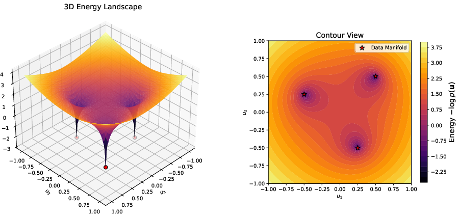
- Marginal energy: The authors define a single energy for noisy data, called the marginal energy. It’s the negative log of a “mixed” probability over all possible noise levels:
- , and .
- Think of as “how likely is this noisy sample u, if we consider every possible noise level t?” The energy is like the height of a landscape; low energy means “more likely.”
- Gradient descent: Models typically “move downhill” in this landscape along the steepest direction (the gradient). But near the true clean image, the usual gradient becomes extremely steep—like an infinitely deep pit—which would normally make the model unstable.
- Riemannian gradient flow (a smart speed limit): The paper shows autonomous models don’t follow the raw steepest path. Instead, they follow a scaled version that uses a local “speed limit” depending on how noisy things are nearby. This scaling is like wearing special shoes that automatically slow you down near cliffs so you don’t fall. In math terms, this is a Riemannian gradient flow with a local conformal metric (a local scale factor).
- Decomposition of the learned rule: The authors break the learned, time-invariant movement rule into three parts:
- A natural gradient term (moving downhill in the marginal energy, but with a smart local scale).
- A transport correction term (a small adjustment that matters when the model isn’t sure about the noise level).
- A simple linear drift (a gentle push that keeps the motion balanced with the overall noise geometry).
- Two situations where uncertainty fades:
- High dimensions: In very high-dimensional spaces (like big images), different noise levels look very different, so the model can guess the noise level from the sample itself.
- Near the clean data: As you get close to the final clean image, only tiny noise levels make sense, so the model’s guess about the noise level becomes very sharp.
Main Findings and Why They Matter
Here are the main results, explained plainly:
- Autonomous models follow a single “marginal energy” landscape: Even without noise-level input, the model is effectively moving downhill on one shared landscape that mixes over all noise levels. This gives a clear purpose to what it is optimizing.
- The raw landscape is dangerously steep near clean images—but the model cancels that danger: The gradient of this energy becomes infinite near the true image, which would usually be unstable. However, the learned model automatically applies a local scale (a “smart brake”) that shrinks steps exactly enough to avoid instability. This turns the infinite pit into a safe attractor.
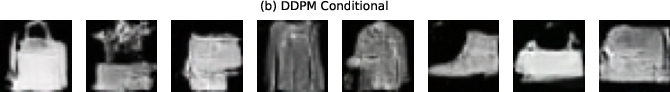
- Stability depends on how you train the model to predict:
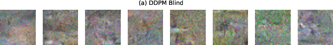
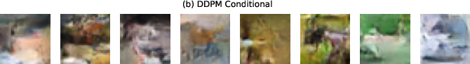
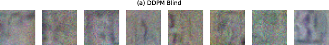
- Noise-prediction parameterizations (like standard DDPM/DDIM “predict the noise”) behave like high-gain amplifiers near low noise: small errors get blown up. This causes blind (autonomous) versions to fail catastrophically.
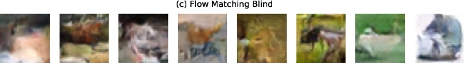
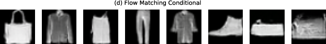
- Velocity-based parameterizations (Flow Matching, Equilibrium Matching) have bounded gain (no amplification), so they naturally absorb uncertainty and remain stable even without noise conditioning.
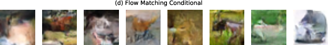
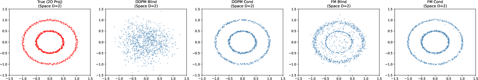
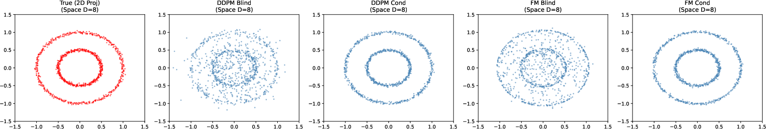
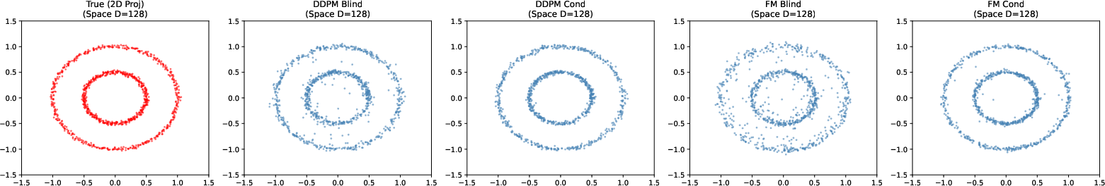
- Experiments confirm the theory:
- Blind DDPM fails in practice (noisy, unstable samples).
- Blind Flow Matching works well, producing clean results similar to models that do get the noise level.
These findings matter because they explain when and why you can safely drop noise conditioning, which can simplify models and sampling.
Implications and Impact
This work suggests a cleaner way to design generative models:
- Autonomous, time-invariant models are not just “denoisers guessing blindly”—they are carefully following a single energy landscape with built-in local safety controls.
- If we use velocity-based training targets, autonomous models can be both simple and stable, avoiding the tricky, unstable behavior of noise-prediction targets when noise conditioning is removed.
- Practically, this can lead to faster, simpler samplers and new architectures that don’t need explicit time/noise inputs, especially for high-dimensional data (like images) or near the final clean solution.
In short: you can build generative models that don’t need to be told the noise level, as long as you train them to predict “how to move” (velocity) rather than “what the noise is.” The geometry makes this safe, and the experiments show it works.
Knowledge Gaps
Knowledge gaps, limitations, and open questions
Below is a consolidated and concrete list of what remains missing, uncertain, or unexplored in the paper, framed as actionable directions for future research.
- Formalize the conformal/Riemannian metric: derive an explicit, data-dependent expression for the local metric beyond a scalar gain (e.g., anistropic, direction-dependent preconditioning distinguishing normal vs. tangential directions to the data manifold), and characterize when isotropic conformal scaling is insufficient.
- Quantify posterior concentration rates: provide non-asymptotic bounds for the rate at which the posterior p(t|u) concentrates (as a function of codimension D−d, curvature, noise schedule, and distance to the manifold), including explicit constants that determine when the transport correction term is negligible.
- Bound the transport correction term: establish computable upper bounds on the covariance-based correction term in the autonomous field decomposition, and identify data/schedule regimes guaranteeing its smallness; develop practical diagnostics to detect when this term is non-negligible in real datasets.
- Dependence on the time prior p(t): analyze how the choice and misspecification of the training prior p(t) shape the marginal energy, its singularity, and stability; characterize optimal or robust p(t) (e.g., over log-SNR) and how to adapt or learn it from data.
- Robustness to schedule mismatch at inference: quantify how deviations between the sampler’s schedule and the training prior p(t) affect stability and sample quality; design correction schemes (e.g., reweighting, inverse-temperature annealing) to mitigate mismatch.
- Beyond affine Gaussian corruption: extend theory to non-Gaussian and signal-dependent noise, non-linear forward processes, and general corruption families; determine conditions under which the Riemannian flow interpretation and stability carry over.
- SDE-based sampling: generalize the stability analysis from deterministic ODE flows to stochastic samplers (Itô/Stratonovich SDEs), including how injected noise interacts with the gain singularities and whether it regularizes or destabilizes autonomous dynamics.
- Discretization and numerical stability: provide step-size conditions, integrator choices, and global error bounds ensuring stable autonomous sampling near t→0 (where stiffness arises), and quantify trade-offs between stability and sample quality.
- Stabilizing noise-prediction parameterizations: investigate principled modifications (e.g., gain clipping, schedule redesign, posterior-corrected targets, variance-aware normalization) that eliminate the “Jensen Gap” amplification and render ε-parameterizations stable in the autonomous regime.
- Constructive training for energy alignment: design explicit objectives/regularizers that enforce alignment with the marginal energy’s natural gradient and control the gain λ, rather than relying on implicit emergence through MSE; compare against dual score/energy learning.
- Empirical measurement of geometric terms: develop estimators to measure in practice the marginal gradient, effective gain, and transport correction from trained models; validate the predicted cancellation of singularities and identify datasets where it fails.
- Applicability in low or modest codimension: characterize the practical codimension thresholds at which autonomous models become reliable; provide empirical tools to estimate intrinsic dimension and predict when blind generation will fail without time conditioning.
- Scaling and modality coverage: validate claims on large-scale, high-resolution benchmarks (e.g., ImageNet 256/512, LAION) and other modalities (audio, video, 3D); assess whether the stability/geometry conclusions hold for diffusion transformers and modern backbones.
- Conditioning beyond noise (e.g., text/image conditioning): analyze whether and how the autonomous/Riemannian framework extends to conditional generation, where additional inputs may alter the geometry and concentration properties.
- Choice of t_min and near-zero regimes: quantify how a finite minimum noise level (t_min) impacts the stiffness of the energy landscape, gradient magnitudes, and training/sampling stability; provide principled methods to pick t_min and schedule tapering.
- Anisotropy near data manifolds: examine whether singularities are directionally concentrated (normal vs. tangential), and test if scalar gains suffice; if not, propose anisotropic gain learning or metric-aware architectures.
- Architectural implications: study which architectural choices (U-Net vs. transformer, normalization layers, residual scaling) facilitate bounded, well-conditioned autonomous fields and reliable gain behavior without time embeddings.
- Generalization and sample complexity: analyze how learning a single autonomous field affects sample complexity and generalization across noise levels; derive conditions under which autonomous models are statistically more/less efficient than time-conditioned ones.
- Hybrid or gated conditioning: explore models that are autonomous in concentrated regimes but selectively condition on t in ambiguous regions (low dimensions or far from the manifold); propose criteria to switch between modes.
- Energy estimation and calibration: investigate whether marginal energy can be estimated/regularized directly (e.g., for OOD detection or likelihood calibration), and how its singularities can be smoothed without sacrificing stability or sample quality.
Practical Applications
Immediate Applications
The paper’s findings enable several deployable changes to current generative, denoising, and restoration workflows by replacing noise-prediction targets with bounded-gain, velocity-based parameterizations and by exploiting the implicit “marginal energy” geometry.
- Healthcare imaging (dose-agnostic denoising and reconstruction)
- Sector: Healthcare
- Use case: Train a single, time-invariant model to denoise MRI/CT/PET scans across varying dose/SNR without explicit noise-level inputs; deploy EqM/Flow Matching samplers to maintain stability.
- Tools/products/workflows: PACS-integrated blind denoisers; radiology pipeline plugins that avoid protocol-specific models.
- Assumptions/dependencies: High-dimensional image data; training data must cover realistic noise priors p(t); velocity-based targets (EDM/Flow Matching/EqM) and step-size control to avoid stiffness near t→0; regulatory validation.
- Smartphone/consumer imaging (ISO-agnostic noise removal)
- Sector: Consumer software & hardware
- Use case: “One denoiser for all ISO” in camera and photo editing apps; remove user-facing “noise level” sliders and auto-infer the noise scale from the image.
- Tools/products/workflows: On-device autonomous denoising filters using FM/EqM; integration into mobile ISPs.
- Assumptions/dependencies: Training with mixed noise conditions (real and synthetic); efficient velocity-based samplers; hardware acceleration.
- Audio noise suppression across SNRs
- Sector: Audio/DSP, Assistive tech
- Use case: Hearing aids, conferencing, and streaming apps deploy a single blind denoiser robust to unknown SNR and environments.
- Tools/products/workflows: Real-time velocity-parameterized architectures; adaptive step-size samplers.
- Assumptions/dependencies: Low-latency implementations; coverage of noise types in training; FM/EqM parameterization to avoid gain blow-ups.
- Remote sensing and microscopy (blind denoising at varying noise/backscatter)
- Sector: Remote sensing, Life sciences
- Use case: Stable, blind denoising for SAR/satellite and fluorescence microscopy where noise varies by scene/acquisition.
- Tools/products/workflows: Cloud geospatial pipelines and instrument control software using autonomous FM/EqM models.
- Assumptions/dependencies: Representative priors p(t); velocity-based targets; QA with stability diagnostics.
- Robust blind image restoration (inpainting, super-resolution, deblocking) with unknown degradation severity
- Sector: Creative tools, Imaging
- Use case: One restoration model handles unknown severity levels (e.g., JPEG quality, blur) by leveraging autonomous fields.
- Tools/products/workflows: Plugins for Photoshop/GIMP/DaVinci; automatic severity-agnostic settings.
- Assumptions/dependencies: Forward degradation models must be incorporated into the unified affine framework; velocity-based training targets.
- ML engineering guideline: replace noise prediction with velocity-based targets in blind settings
- Sector: Software/ML infra
- Use case: Update diffusion libraries and internal frameworks to prefer FM/EqM targets for time-invariant networks; deprecate autonomous noise-prediction heads.
- Tools/products/workflows: Diffusers-like APIs with
parameterization="velocity"by default whentis not provided; sampler presets with bounded gain. - Assumptions/dependencies: Backwards compatibility; training re-runs; schedule prior selection.
- Stability diagnostics and safeguards in production sampling
- Sector: Software/ML ops
- Use case: Instrument samplers with runtime checks on effective gain
nu(t)and drift perturbationΔv = |nu(t)| * ||f*(u) − f*_t(u)||; auto-adjust step size or switch parameterizations when thresholds are exceeded. - Tools/products/workflows: “Bounded-gain sampler” modules; dashboards reporting estimated Jensen Gap amplification.
- Assumptions/dependencies: Estimating or bounding
||f*(u) − f*_t(u)||via proxies; integration with monitoring.
- Model size and API simplification for edge deployment
- Sector: Edge/embedded
- Use case: Remove time-embedding pathways to reduce parameters and simplify APIs; keep time-dependent scaling only in the sampler.
- Tools/products/workflows: Lightweight U-Nets or transformers without time-conditioning; schedule tables in firmware.
- Assumptions/dependencies: No loss in fidelity requires velocity-based targets and well-tuned schedules; memory-compute tradeoffs.
- Academic benchmarking and teaching materials
- Sector: Academia
- Use case: New benchmarks for autonomous (noise-unconditional) generation; labs demonstrating stability differences between parameterizations.
- Tools/products/workflows: Open-source notebooks that toggle between noise-, signal-, and velocity-targets; concentration probes based on norm geometry.
- Assumptions/dependencies: Datasets spanning noise ranges; simple toy datasets to visualize high-dimensional concentration.
Long-Term Applications
These directions leverage the paper’s geometric insights (marginal energy, Riemannian gradient flow, bounded-gain conditions) but require further research, scaling, or integration.
- Riemannian-preconditioned samplers and adaptive metrics
- Sector: Software/ML research
- Use case: Design integrators that explicitly estimate/track the local conformal metric implied by posterior noise variance to accelerate and stabilize sampling.
- Tools/products/workflows: Metric-aware ODE/SDE solvers; adaptive preconditioning layers.
- Assumptions/dependencies: Reliable local metric estimation; theoretical guarantees under model error.
- Unified blind inverse problem solvers (multiple unknown degradations)
- Sector: Imaging, Scientific computing
- Use case: Single autonomous model for unknown combinations of noise, blur, compression, and sensor artifacts using an extended marginal energy over multiple latent nuisance variables.
- Tools/products/workflows: Generative solvers that marginalize over degradation priors; plug-and-play with physics-informed forward models.
- Assumptions/dependencies: Accurate priors over degradations; training data breadth; scalable inference.
- Standardization and compliance in clinical deployments
- Sector: Policy/Healthcare
- Use case: Guidance documents recommending bounded-gain (velocity/EqM) parameterizations for blind denoising to prevent instability; test protocols focused on drift amplification risks.
- Tools/products/workflows: Certification checklists; regulatory audits for sampler stability.
- Assumptions/dependencies: Consensus across stakeholders; validation datasets representing dose/noise diversity.
- Energy-based controllable generation via marginal energy shaping
- Sector: Creative/Media, Robotics
- Use case: Shape or compose marginal energies (e.g., with task-specific priors) to steer autonomous flows for style, content, or constraint satisfaction; apply to robot perception/planning with uncertainty-aware flows.
- Tools/products/workflows: Energy modulators and constraint layers; control-toolbox integrations.
- Assumptions/dependencies: Methods to edit/compose energies without destabilizing the flow; safety analyses.
- Multi-modal and sensor-fusion models with unknown per-modality noise
- Sector: Robotics, AR/VR, Autonomous systems
- Use case: Autonomous fields that marginalize over different noise levels per modality (e.g., LiDAR/RGB/IMU), yielding stable fusion without explicit per-sensor calibration.
- Tools/products/workflows: Cross-modal FM/EqM training; fusion samplers with modality-specific gains.
- Assumptions/dependencies: Identifiability of per-modality noise; synchronized multi-sensor datasets.
- Continual and federated adaptation of noise priors p(t)
- Sector: ML systems, Privacy
- Use case: Online update of the noise-level prior from incoming data, enabling blind denoisers to adapt to deployment domains without raw data sharing.
- Tools/products/workflows: Federated prior estimation; lightweight posterior concentration probes.
- Assumptions/dependencies: Privacy constraints; mechanisms to prevent catastrophic instability during updates.
- Hardware-aware co-design (SAMPLER × PARAMETERIZATION)
- Sector: Semiconductor, Edge AI
- Use case: Co-design accelerators that exploit time-invariant networks and bounded-gain samplers; optimize memory bandwidth by removing time embeddings.
- Tools/products/workflows: Instruction sets for metric-aware solvers; compiler passes for autonomous flows.
- Assumptions/dependencies: Stable schedules at reduced precision; calibration pipelines.
- Theoretical tools and audits for risk management
- Sector: Policy/Compliance, ML governance
- Use case: “Jensen Gap auditors” that score deployment risk based on estimated amplification factors; red-team tests around t→0 stiffness.
- Tools/products/workflows: Risk scoring reports; CI checks during model updates.
- Assumptions/dependencies: Practical proxies for posterior uncertainty and amplification; accepted thresholds.
- Generalized marginal-energy training for non-image domains
- Sector: Finance, Energy, Bioinformatics
- Use case: Autonomous generative models for tabular, time-series, or molecular data with unknown noise or perturbation levels; stable sampling via bounded-gain flows.
- Tools/products/workflows: Domain-specific priors and augmentation pipelines; interpretable drift diagnostics.
- Assumptions/dependencies: Adequate intrinsic-vs-ambient dimensionality for concentration; domain-adapted schedules.
Notes on feasibility across applications:
- Stability requires bounded-gain parameterizations (velocity/signal) and careful integrator design; autonomous noise-prediction is structurally unstable due to gain ∝ 1/b(t).
- Posterior concentration (high ambient vs low intrinsic dimension or near-manifold proximity) underpins practical success; training data and priors p(t) must reflect deployment conditions.
- For regulated domains, explicit validation of stability near low-noise regimes and drift amplification controls is essential.
Glossary
- Affine diffusion process: A diffusion/noising process whose forward dynamics are affine functions of the clean data and noise via schedule functions. "our framework is generalized across arbitrary affine diffusion processes and learning targets."
- Affine formulation: A unified representation of the forward process as a linear combination of signal and noise controlled by schedules. "we adopt the unified affine formulation proposed by \citet{sun2025isnoise}."
- Autonomous generative models: Models that learn a single, time-invariant vector field without explicit noise-level conditioning. "Autonomous (noise-agnostic) generative models, such as Equilibrium Matching and blind diffusion, challenge the standard paradigm"
- Bounded-gain condition: A stability property where the sampler’s multiplicative gain on the model output remains bounded, preventing error amplification. "because they satisfy a bounded-gain condition that absorbs posterior uncertainty into a smooth geometric drift."
- Codimension: The difference between ambient and intrinsic dimensions, often governing the dominance of orthogonal noise components. "Because the codimension is large, the magnitude of this orthogonal noise dominates the total norm."
- Conformal metric: A position-dependent scalar metric scaling that preconditions gradients geometrically. "a local conformal metric that perfectly counteracts the geometric singularity"
- Data manifold: The (typically low-dimensional) subset of ambient space on which clean data lie. "near the data manifold where gradients typically diverge?"
- DDPM (Denoising Diffusion Probabilistic Models): A class of diffusion models trained with variance-preserving forward processes and noise prediction. "Denoising Diffusion Probabilistic Models (DDPM)~\cite{ho2020denoising}"
- Dirac delta: A point-mass distribution modeling perfect concentration at a single value. "collapses to a Dirac delta centered at an implicit estimate ."
- Drift Perturbation Error: The deviation between autonomous and oracle sampler velocities due to target mismatch. "The structural stability is determined by the Drift Perturbation Error , which measures the deviation"
- Effective gain: The time-dependent scalar factor multiplying the model output within the sampler dynamics. "The Drift Perturbation Error is the product of the Effective Gain and the estimation error."
- Energy landscape: The potential surface defined by an energy function whose gradients drive dynamics. "The Singular Geometry of the Marginal Energy Landscape."
- Energy-based learning: Training approaches that shape an energy function over inputs whose gradients guide inference. "While the framework of energy-based learning is well-established"
- Equilibrium Matching (EqM): An autonomous generative modeling framework that aligns with a marginal energy objective. "Equilibrium Matching (EqM)\cite{wang2025equilibrium}."
- Flow Matching: A velocity-based transport formulation that learns trajectories between distributions. "Flow Matching~\cite{lipman2023flow}"
- High-dimensional concentration: The phenomenon that probability mass concentrates (e.g., on shells) in high dimensions, aiding implicit noise inference. "high-dimensional concentration allows these models to implicitly estimate noise levels from corrupted observations,"
- Jensen Gap: The discrepancy arising from applying a nonlinear function before averaging versus after, here amplifying errors under averaging. "We identify a ``Jensen Gap'' in noise-prediction parameterizations that acts as a high-gain amplifier for estimation errors,"
- JKO scheme: The Jordan–Kinderlehrer–Otto variational time-discretization of gradient flows such as Fokker–Planck. "This connects EqM to the fundamental JKO scheme \cite{jordan1998variational}"
- Langevin-type SDE discretizations: Numerical schemes based on Langevin dynamics used to implement stochastic sampling. "their analysis focuses primarily on specific Langevin-type SDE discretizations,"
- Linear drift: A term proportional to the state (u) that models global expansion/contraction in the vector field. "and a linear drift."
- Marginal energy: The negative log-density of noisy data marginalized over unknown noise levels. "a specific form of Riemannian gradient flow on this Marginal Energy."
- Mean Squared Error (MSE): A training loss equal to the expected squared difference between predictions and targets. "by minimizing the Mean Squared Error (MSE):"
- Natural gradient: A Riemannian gradient that accounts for the underlying metric, yielding preconditioned descent. "implements a natural gradient descent on the marginal energy."
- Nearest-neighbor lookup: A degenerate estimator that selects the closest sample, arising in unsmoothed energy/score formulations. "degenerates into a nearest-neighbor lookup."
- Noise-Blind Denoising: Denoising/generation without providing the noise level to the model at training or inference. "Noise-Blind Denoising."
- Potential well: A low-energy region attracting trajectories; here, it can be singularly deep near the data manifold. "converting an infinitely deep potential well into a stable attractor."
- Riemannian gradient flow: Gradient descent dynamics defined with respect to a Riemannian metric rather than the Euclidean one. "a specific form of Riemannian gradient flow on this Marginal Energy."
- Riemannian preconditioner: A metric-based scaling that stabilizes and preconditions gradient dynamics. "we show that autonomous flow models resolve it implicitly via a Riemannian preconditioner."
- Score-based models: Models that learn the score (gradient of log-density) to drive sampling dynamics. "Score-based models~\cite{song2019generative,song2020improved,vincent2011connection}"
- Score-based stochastic differential equations (SDEs): SDE formulations whose drifts/diffusions are tied to learned score fields. "score-based stochastic differential equations (SDEs)"
- Signal-to-noise ratio (SNR): The ratio of signal power to noise power, indicating corruption level in the forward process. "the signal-to-noise ratio (SNR) at time is"
- Structural stability: Robustness of sampling dynamics to perturbations in the learned field or parameters. "We also establish the structural stability conditions for sampling with autonomous models."
- Transport correction: A covariance-based correction term accounting for mixing over noise levels in the autonomous field. "a transport correction (covariance) term,"
- Tweedie’s formula: An identity connecting the posterior mean denoiser to the score of the noisy distribution. "we use Tweedie's formula \cite{robbins1992empirical,efron2011tweedie} to express the conditional score"
- Variance preserving diffusion processes: Forward processes where signal and noise variances sum to a constant over time. "variance preserving diffusion processes"
- Velocity-based parameterizations: Targets predicting velocity instead of noise, yielding bounded gains and stable sampling. "velocity-based parameterizations are inherently stable"
Collections
Sign up for free to add this paper to one or more collections.