Differentiating through Stochastic Differential Equations: A Primer
Abstract: Dynamical systems are essential to model various phenomena in physics, finance, economics, and are also of current interest in machine learning. A central modeling task is investigating parameter sensitivity, whether tuning atmospheric coefficients, computing financial Greeks, or optimizing neural networks. These sensitivities are mathematically expressed as derivatives of an objective function with respect to parameters of interest and are rarely available analytically, necessitating numerical methods for approximating them. While the literature for differentiation of deterministic systems is well-covered, the treatment of stochastic systems, such as stochastic differential equations (SDEs), in most curricula is less comprehensive than the subtleties arising from the interplay of noise and discretization require. This paper provides a primer on numerical differentiation of SDEs organized as a two-tale narrative. Tale 1 demonstrates differentiating through discretized SDEs, known the discretize-optimize approach, is reliable for both Itô and Stratonovich calculus. Tale 2 examines the optimize-discretize approach, investigating the continuous limit of backward equations from Tale 1 corresponding to the desired gradients. Our aim is to equip readers with a clear guide on the numerical differentiation of SDEs: computing gradients correctly in both Itô and Stratonovich settings, understanding when discretize-optimize and optimize-discretize agree or diverge, and developing intuition for reasoning about stochastic differentiation beyond the cases explicitly covered.
Paper Prompts
Sign up for free to create and run prompts on this paper using GPT-5.
Top Community Prompts
Explain it Like I'm 14
Overview
This paper is a friendly guide to a tricky but important task: how to correctly compute “sensitivities” (gradients) when your system is driven by randomness. These systems are called stochastic differential equations (SDEs). The authors show how to:
- Safely differentiate through computer simulations of SDEs (the way most people actually compute).
- Understand when a more “theory-first” approach works or fails.
- Do this both for the two main kinds of SDE math: Itô and Stratonovich calculus.
They illustrate everything with clear examples from finance (like the Black–Scholes model for stock prices) and give practical rules you can follow.
What questions are the authors asking?
In simple terms, they ask:
- If a system evolves with random bumps and wiggles, how does the final outcome change when we tweak the starting point or other parameters? That “how much it changes” is the gradient.
- What is the safest way to compute these gradients on a computer?
- Do the “computer gradients” match the “perfect, continuous-time” gradients as we make the time steps smaller and smaller?
- Does the answer depend on which kind of stochastic calculus we use (Itô vs Stratonovich)?
How did they study it? Key ideas and methods
To keep things concrete, picture this: you’re walking along a path where, at each step, random gusts of wind push you around. You want to know how changing your starting spot (or some setting like “windiness”) affects where you end up. That’s a gradient.
Modeling randomness with SDEs
- An SDE is like an ordinary differential equation (ODE), but with randomness added.
- Itô calculus and Stratonovich calculus are two ways to define “how randomness enters” each tiny step. Think of them as two different rules for measuring the gust of wind:
- Itô: measure using information at the beginning of each step (left endpoint).
- Stratonovich: measure in a more “balanced” way, roughly like averaging across the step (midpoint).
Two strategies for getting gradients
There are two classic approaches:
- Discretize–then–Optimize (DTO):
- First, approximate the SDE by taking small time steps (like stepping stones).
- Then run automatic differentiation (backpropagation) through those steps to get the gradient.
- This is exactly what deep learning frameworks do: simulate forward, then backprop.
- Optimize–then–Discretize (OTD):
- First, write down a “perfect” continuous-time equation for the gradient.
- Then discretize that gradient equation and compute it numerically.
The paper tells “two tales,” one for each approach.
Numerical stepping rules (the simulators)
- For Itô SDEs, they use the Euler–Maruyama method (a standard, simple stepping rule).
- For Stratonovich SDEs, they use the Heun method (a predictor–corrector step that matches Stratonovich’s midpoint spirit).
Choosing the right stepping rule matters. Using the wrong one can point you to the wrong kind of SDE in the limit.
How gradients are actually computed
- Pathwise gradients: For each simulated random path, you can differentiate the final value with respect to the input (start or parameter).
- Then average these pathwise gradients across many random paths (Monte Carlo).
- Reverse-mode automatic differentiation (aka backpropagation or the “adjoint” method) computes this efficiently: instead of pushing entire matrices forward, it pulls one vector backward through time. This is much faster and is what ML libraries do under the hood.
Parameters and running costs
- If you care about a parameter (like volatility in finance), you can treat it as an extra “state” that doesn’t change over time. Then backpropagation automatically gives you its gradient.
- If your objective includes a “running cost” (something that accumulates over time, like total energy used), add another state that integrates this cost as you go. Then you can still use the same gradient machinery.
Experiments: Black–Scholes and CEV
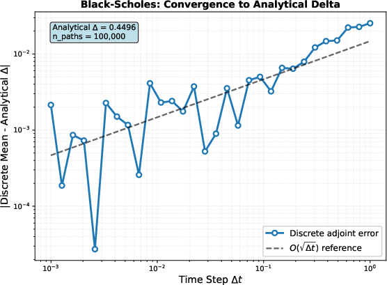
- Black–Scholes (stock price model): a classic Itô SDE with a known solution, great for checking that the computed gradients are correct. The authors show that the DTO gradients converge as you take smaller time steps, until you hit the usual Monte Carlo noise.
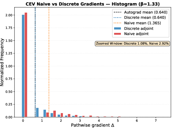
- CEV (Constant Elasticity of Variance): a variation where the noise depends more strongly on the current state. This example reveals when a “naive” method gives seriously biased gradients.
What did they find and why does it matter?
Here are the main takeaways, explained simply:
- Discretize–then–Optimize (DTO) is safe for both Itô and Stratonovich SDEs. If you simulate with the correct scheme (Euler–Maruyama for Itô, Heun for Stratonovich) and then backpropagate through your simulation, you’ll get correct gradients for the discretized problem. As you shrink the time step, these estimates converge as expected.
- A naive Optimize–then–Discretize (OTD) approach can fail for Itô SDEs. If you try to write down a continuous-time backward equation for the gradient and then discretize it “like an ODE,” you can end up biased. Why? Because Itô calculus is very sensitive to when you measure the random increment (“left endpoint” matters). Mixing up these timing rules breaks the math.
- Sometimes the naive Itô OTD looks okay by accident. In Black–Scholes, the diffusion’s derivative is constant, so the naive and correct methods accidentally match. But in the CEV model, where that derivative depends on the state, the naive method gives gradients that are way off (even more than twice as large on average in the authors’ test) and can be unstable.
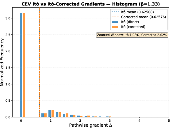
- OTD works naturally in the Stratonovich setting. With Stratonovich calculus (which aligns with midpoint/trapezoid-like rules), the discrete adjoints do converge to a well-defined continuous “backward SDE for the gradient.” This agrees with modern theory (rough path theory) and gives a solid foundation if you prefer to “derive first, discretize later.”
- Practical performance checks out. In Black–Scholes tests, the error shrinks at the expected rate for Euler–Maruyama (like the square root of the time step), then levels off due to Monte Carlo randomness—just as theory predicts.
Why this matters:
- Many real problems in physics, finance, and machine learning need gradients through randomness (for tuning models, computing sensitivities like “Greeks,” or training neural SDEs).
- This paper tells you which buttons you can press with confidence using standard tools (AD/backprop), and when you need to be careful about the math of randomness.
Implications and potential impact
- For practitioners: The simplest safe recipe is “simulate with the right scheme and backprop through the simulation.” This is DTO, and it works for both Itô and Stratonovich.
- For theorists or when designing custom solvers: If you want to derive continuous-time adjoint equations and then discretize them (OTD), work in the Stratonovich setting; its midpoint nature makes the limits behave well.
- For finance: Computing Greeks by backpropagating through a Monte Carlo SDE simulator is reliable if you use the correct stepping rule. Beware shortcuts that assume ODE-like logic in Itô settings—those can be biased unless special structure (like Black–Scholes) saves you.
- For machine learning: Training neural SDEs is feasible with off-the-shelf automatic differentiation by differentiating through the SDE solver, averaging over sample paths, and optionally augmenting states to include parameters and running costs.
- Big picture: The paper sharpens intuition about how randomness and discretization interact. The “endpoint” where you evaluate random increments matters. Knowing this helps you pick methods that are both correct and efficient.
In short, the paper provides a clear, practical playbook: use DTO for Itô and Stratonovich; if you need OTD, prefer Stratonovich; and always respect the timing rules of randomness when designing your algorithms.
Knowledge Gaps
Knowledge gaps, limitations, and open questions
Below is a single, concrete list of gaps and open questions that remain unresolved in the paper. Each item is phrased to enable targeted follow-up by future researchers.
- Precise interchange conditions: Specify and prove the minimal regularity and integrability assumptions under which differentiation and expectation can be interchanged for SDE objectives, especially with nonsmooth terminal payoffs such as .
- Existence and differentiability of SDE flows: State and verify conditions (Lipschitz, linear growth, bounded derivatives) that guarantee pathwise differentiability of w.r.t. and parameters, including edge cases (e.g., CEV with non-Lipschitz diffusion near zero, absorbing boundaries).
- Gradient convergence theory: Establish strong/weak convergence rates for discrete adjoint gradients under Euler–Maruyama (Itô) and Heun (Stratonovich), and provide error decompositions separating discretization bias from Monte Carlo variance.
- Optimize–discretize for Itô SDEs: Develop a rigorous continuous-time adjoint framework for Itô dynamics (if possible), clarifying whether a backward Itô SDE, an anticipating/Skorokhod integral formulation, Malliavin-weight representations, or FBSDE-based adjoints are required; identify conditions under which the discrete adjoint has a continuous limit.
- Stratonovich adjoint discretization: Derive and validate practical time-discretization schemes for the continuous backward Stratonovich adjoint SDE (beyond heuristic midpoint intuition), including stability and convergence guarantees.
- Multidimensional non-commutative noise: Analyze the impact of Lévy area terms for Stratonovich SDEs on gradient computation; determine when Heun is sufficient and when iterated integrals are needed, and design adjoint-capable schemes that handle non-commuting vector fields.
- Higher-order methods: Extend adjoint derivations to Milstein and stochastic Runge–Kutta schemes (Itô and Stratonovich) and compare their gradient accuracy, cost, and stability against Euler–Maruyama/Heun.
- Parameter sensitivities in Stratonovich: Provide explicit adjoint recursions and continuous-time formulas for gradients w.r.t. parameters in Stratonovich SDEs (augment-as-state strategy was outlined only for Itô).
- Running costs in continuous time: Derive the continuous adjoint for objectives with running costs (integral functionals) and give a discretization that matches the forward scheme (Itô vs. Stratonovich), including error analysis.
- Path-dependent and stopping-time objectives: Address gradients for barrier/knock-out options, American options, and other path-dependent payoffs or stopping times, where differentiability and measurability issues arise; propose robust estimators (e.g., smoothed payoffs, likelihood ratio methods).
- Jump diffusions and Lévy noise: Extend the discretize–optimize and optimize–discretize frameworks to SDEs with jumps, specifying adjoint recursions that incorporate Poisson/Lévy jumps and clarifying the role of Itô vs. Stratonovich in this setting.
- Gradient variance and stability: Quantify and control the variance and tail behavior of pathwise gradient estimators (e.g., heavy tails observed for naive schemes), and evaluate variance-reduction methods (antithetic sampling, control variates, stratification) tailored to adjoint gradients.
- Adaptive timestepping and stiffness: Study how adaptive solvers and stiff dynamics affect adjoint accuracy and stability (both discrete and continuous adjoints), and propose checkpointing/memory strategies for long horizons.
- Correlated and time-dependent noise: Generalize derivations to correlated Brownian motions and time/state-dependent diffusion matrices; characterize how correlation structure enters the adjoint and impacts convergence.
- Second-order sensitivities: Formulate and analyze discrete/continuous adjoint methods for second derivatives (e.g., Gamma, Hessians) including reverse-on-forward strategies and their variance/complexity trade-offs.
- Neural SDEs and large-scale training: Provide algorithms and guarantees for memory-efficient adjoints in neural SDE training (analogous to continuous adjoint for neural ODEs), and assess when Stratonovich optimize–discretize can reduce memory vs. backprop through the forward solver.
- Alternative gradient estimators: Compare pathwise adjoints to Malliavin-weight (likelihood ratio) estimators for Greeks and parameter inference, including bias–variance trade-offs and scenarios where each is preferable.
- Itô–Stratonovich conversion and drift corrections: Explicitly demonstrate how gradient formulas change under Itô↔Stratonovich conversion (e.g., Itô correction terms) and identify when discretize–optimize is “calculus-aware” vs. when scheme–calculus mismatches induce bias.
- Robustness to nonsmooth payoffs: Investigate gradient existence and numerical stability for objectives with kinks/plateaus (e.g., options), and assess smoothing or subgradient approaches with provable error bounds.
- Error budgets and practical guidance: Provide principled guidelines for selecting timestep sizes and path counts that meet target gradient accuracies, with explicit error budget splits (discretization vs. sampling).
- Boundary/degeneracy handling: Analyze gradient behavior near absorbing/reflecting boundaries or degeneracy in diffusion (e.g., ), and design adjoint-compatible schemes that respect boundary conditions.
- Deterministic–stochastic hybrid systems: Extend methodology to models with mixed deterministic controls and stochastic disturbances (e.g., controlled SDEs), including adjoints for control inputs and constraints.
- Calibration and likelihood gradients: Address parameter estimation from discrete observations by deriving adjoints for the log-likelihood (via Girsanov or score-based methods) and quantify estimator properties under misspecification.
- Numerical verification breadth: Broaden experiments beyond Black–Scholes Delta to include other Greeks (Gamma, Vega, Theta, Rho), Stratonovich cases, multidimensional noise, and models with state-dependent diffusion (e.g., CEV with ), reporting systematic convergence and variance analyses.
- Implementation details of terms: Clarify how higher-order terms (e.g., , , ) are handled in AD frameworks in practice (e.g., treatment of ), and assess their impact on gradient bias/variance.
Practical Applications
Overview
The paper presents a practical primer for differentiating through stochastic differential equations (SDEs), establishing when and how to compute correct gradients for objectives dependent on stochastic dynamics. It provides concrete recipes for:
- Discretize-then-optimize (safe for both Itô and Stratonovich SDEs with appropriate schemes).
- Optimize-then-discretize (safe in Stratonovich via a backward Stratonovich SDE; generally unsafe in Itô unless special conditions hold).
- Handling parameter sensitivities and running costs via state augmentation.
- Validating and implementing adjoint-based gradients in numerical practice (notably for the Black–Scholes and CEV models).
Below are actionable applications grouped by deployment horizon.
Immediate Applications
The following items can be deployed now using the paper’s methods and code patterns (e.g., Euler–Maruyama for Itô and Heun for Stratonovich, reverse-mode AD, augmented states for parameters/running costs).
- Finance — Monte Carlo Greeks with unbiased adjoints
- Use case: Compute Delta/Vega/Rho/Theta/Gamma for vanilla and exotic options under SDE models (Black–Scholes, CEV, local volatility).
- Workflow/product: Adjoint-based “Greeks engine” that simulates paths and backpropagates through Euler–Maruyama (Itô) or Heun (Stratonovich), averages pathwise gradients, and integrates with pricing/risk systems.
- Assumptions/dependencies:
- Choose discretization to match modeling calculus: Euler–Maruyama (Itô), Heun (Stratonovich).
- Interchange of differentiation and expectation requires smooth integrands; non-smooth payoffs (max) may need smoothing or alternative estimators (e.g., likelihood-ratio, Malliavin).
- Avoid naive optimize-then-discretize for Itô when diffusion Jacobian depends on state (as in CEV)—it yields biased gradients.
- Finance — Model calibration via gradient-based optimization
- Use case: Calibrate drift/diffusion parameters (e.g., volatility surface in local vol/CEV models) by minimizing discrepancy to market data.
- Workflow/product: Treat parameters as augmented constant states; run adjoint recursion to compute ∇θJ and update with standard optimizers (Adam/L-BFGS).
- Assumptions/dependencies: Sufficient differentiability of drift/diffusion w.r.t. parameters; Monte Carlo variance control (antithetic sampling, control variates).
- Software/ML — Differentiable SDE layers for deep learning
- Use case: Train neural SDEs and continuous-time stochastic models (e.g., time-series forecasting, generative modeling) inside PyTorch/JAX/TensorFlow.
- Workflow/product: Library module offering:
- Forward simulators (Euler–Maruyama, Heun).
- Reverse-mode adjoints for terminal and running costs.
- Parameter augmentation for end-to-end training.
- Assumptions/dependencies: Correct AD integration with stochastic simulators; reproducible random number streams; memory/compute constraints for long horizons.
- Control/Robotics — Sensitivity-based design under stochastic perturbations
- Use case: Optimize controller gains or policies for systems with sensor/actuator noise using gradient information from SDE simulators.
- Workflow/product: Stochastic MPC or policy tuning loop where adjoint gradients inform parameter updates; use Stratonovich+Heun when modeling physical noise with chain-rule consistency.
- Assumptions/dependencies: Accurate noise modeling choice (Itô vs Stratonovich); consistent discretization; cost/regulator differentiability.
- Energy/Commodities — Pricing and hedging with adjoint sensitivities
- Use case: Compute sensitivities for energy derivatives under mean-reverting or regime-switching SDEs and calibrate to historical prices.
- Workflow/product: Risk analytics pipelines leveraging adjoint gradients for scenario analysis and hedge optimization.
- Assumptions/dependencies: Model fit to market microstructure; adequate Monte Carlo sampling and variance reduction.
- Scientific computing/Academia — Teaching and reproducible labs
- Use case: Course modules in stochastic processes, quantitative finance, and scientific computing demonstrating discrete adjoints for SDEs.
- Workflow/product: Adopt the provided GitHub code; include Stratonovich vs Itô differentiation labs showing endpoint evaluation subtleties and convergence behavior.
- Assumptions/dependencies: Students’ background in ODE/SDE numerics and AD; compute resources for Monte Carlo experiments.
- Risk and compliance — Stress testing with sensitivity diagnostics
- Use case: Quantify the impact of parameter/initial condition shifts on risk measures (VaR, ES) by differentiating SDE-based risk models.
- Workflow/product: Reporting tools that compute ∂risk/∂inputs via adjoints to support internal controls and regulatory submissions.
- Assumptions/dependencies: Smoothness of risk aggregations; correct gradient estimation under tail events—may require variance reduction and robust estimators.
Long-Term Applications
These require further research, scaling, or methodological development (e.g., rough paths-backed adjoint solvers, handling non-smooth payoffs robustly, large-scale deployment).
- Standardized optimize-then-discretize adjoint solvers for Stratonovich SDEs
- Sector: Software/ML, Robotics, Physics.
- Product: A robust backward Stratonovich SDE integrator (with rough path foundations) that interoperates with forward Heun schemes and supports complex multi-dimensional noise.
- Dependencies: Implementation of backward Stratonovich adjoints; rough path numerics; stability proofs and benchmarks.
- Bias-safe Itô adjoint frameworks
- Sector: Finance, Engineering.
- Product: Hybrid gradient estimators combining discretize-then-optimize adjoints with Malliavin/likelihood-ratio methods for state-dependent diffusion and non-smooth payoffs.
- Dependencies: Estimator selection logic that detects state-dependent diffusion Jacobians and payoff non-smoothness; variance reduction tooling.
- Large-scale, real-time risk systems on GPU/TPU
- Sector: Finance.
- Product: High-throughput adjoint Monte Carlo for Greeks and calibration across portfolios; integration with intraday risk analytics.
- Dependencies: GPU-friendly SDE simulators with reproducible RNG; memory-efficient checkpointing for adjoints; streaming data pipelines.
- Healthcare/biostatistics — Gradient-based parameter inference in stochastic physiology models
- Sector: Healthcare.
- Product: Patient-specific parameter estimation in stochastic PK/PD or disease progression models using adjoint sensitivities; real-time decision support.
- Dependencies: Model validation against clinical data; careful treatment of observation noise and likelihood formulations; regulatory validation.
- Climate and macroeconomics — Policy scenario calibration and sensitivity analysis
- Sector: Policy, Energy, Economics.
- Product: SDE-based scenario tools where adjoint gradients inform policy levers (e.g., carbon pricing impact, shock propagation).
- Dependencies: Credible stochastic models of macro/earth systems; tractable cost functionals and data assimilation pipelines.
- SPDEs and high-dimensional stochastic systems
- Sector: Scientific computing, Energy, Engineering.
- Product: Extending adjoint differentiation to stochastic partial differential equations (e.g., turbulence models) for design and control.
- Dependencies: New numerical schemes and adjoint derivations for SPDEs; scalable solvers; rigorous convergence guarantees.
- Auto-differentiable SDE tooling ecosystems
- Sector: Software/ML.
- Product: Unified libraries that:
- Automatically choose Itô/Stratonovich discretization and adjoint strategy.
- Offer plug-and-play running cost augmentation and parameter-state coupling.
- Provide diagnostics (bias checks, endpoint evaluation warnings).
- Dependencies: Community standards, test suites, and integration with mainstream ML frameworks.
- Educational standards and certification
- Sector: Academia, Industry training.
- Product: Certification tracks and curricula on differentiating SDEs (with endpoint evaluation, scheme selection, adjoint correctness) for quants/data scientists/engineers.
- Dependencies: Industry-academic collaboration; canonical datasets and benchmarks.
Notes on Assumptions and Dependencies
- Modeling calculus matters:
- Itô: Use Euler–Maruyama and discretize-then-optimize; optimize-then-discretize is generally biased when diffusion Jacobian depends on the state.
- Stratonovich: Use Heun and either discretize-then-optimize or (with further theory) optimize-then-discretize via backward Stratonovich SDE.
- Smoothness and interchange of expectation and differentiation:
- The paper assumes smooth terminal costs; in practice, non-smooth payoffs require care (e.g., smoothing, likelihood-ratio/Malliavin methods).
- Monte Carlo considerations:
- Variance reduction (antithetic sampling, control variates) may be necessary for reliable gradients.
- Convergence rates depend on scheme (e.g., O(√Δt) for Euler–Maruyama).
- Implementation:
- Reverse-mode AD is computationally advantageous for high-dimensional states.
- Store Brownian increments and intermediate states for correct adjoint propagation.
- Physical systems:
- Stratonovich often matches physical modeling (chain rule holds); choose schemes accordingly.
- Validation:
- Benchmark adjoint gradients against analytical solutions (when available) and compare to alternative estimators to detect bias.
Glossary
- Adjoint state: The auxiliary variable that evolves backward to accumulate gradient information for sensitivity analysis. "continuous adjoint state"
- Automatic differentiation: A computational technique that applies the chain rule to compute derivatives of programs efficiently. "via automatic differentiation"
- Backpropagation: The reverse-mode automatic differentiation procedure that computes gradients by propagating sensitivities backward through computations. "reverse-mode automatic differentiation (backpropagation)"
- Backward SDE: A stochastic differential equation formulated backward in time, often used for adjoint processes in optimize–discretize. "backward SDE"
- Black--Scholes model: A financial SDE model for stock prices under geometric Brownian motion, used for option pricing. "Black--Scholes model"
- Brownian increments: Gaussian random variables approximating the increments of Brownian motion over time steps in numerical schemes. "Brownian increments "
- Brownian motion: A continuous-time stochastic process with independent, normally distributed increments used to model noise. "Brownian motion"
- Constant Elasticity of Variance (CEV) model: An SDE where volatility scales with a power of the state, generalizing Black–Scholes. "Constant Elasticity of Variance (CEV) model"
- Controlled differential equations: A class of differential equations driven by rough signals, central to rough path theory. "controlled differential equations"
- Delta: An option Greek measuring sensitivity of the option price to the current stock price. "the Greek "
- Diffusion: The stochastic component of an SDE that multiplies the Brownian motion term. "is the diffusion"
- Discretize-optimize: The approach of discretizing the dynamics first and then differentiating the resulting discrete objective. "discretize-optimize approach"
- Drift: The deterministic component of an SDE that governs the average direction of the state’s evolution. "is the drift"
- Euler-Maruyama scheme: A standard explicit time-stepping method for simulating It^{o} SDEs. "Euler-Maruyama scheme"
- European call option: A financial derivative giving the right to buy the underlying asset at maturity for a fixed strike price. "European call option"
- Forward-mode differentiation: An automatic differentiation mode that propagates derivatives forward with the computation. "Using forward-mode differentiation"
- Gamma: An option Greek measuring the curvature (second derivative) of the option price with respect to the stock price. "Gamma & "
- Geometric Brownian motion: A multiplicative-noise model for asset prices where the logarithm of the price follows Brownian motion. "under geometric Brownian motion"
- Greeks: Sensitivities of option prices with respect to underlying parameters such as price, volatility, time, and interest rate. "Greeks"
- Heun scheme: A stochastic predictor–corrector method that converges to Stratonovich SDEs (the trapezoidal/midpoint analogue). "Heun scheme"
- It^{o} calculus: A framework for stochastic integration and differentiation using left-endpoint evaluation of stochastic integrals. "It^{o} calculus"
- It^{o} SDEs: Stochastic differential equations interpreted in the It^{o} sense with non-anticipative integrals. "It^{o} SDEs"
- Jacobian: The matrix of first-order partial derivatives used to propagate sensitivities through time-stepping updates. "one-step Jacobian"
- Lorenz-63 model: A classic chaotic ODE system used to model atmospheric convection. "Lorenz-63 model"
- Monte Carlo: A sampling-based numerical method for estimating expectations and sensitivities via many random trajectories. "Monte Carlo paths"
- Neural ODEs: Machine learning models where neural networks define continuous-time ODE dynamics. "neural ODEs"
- Neural SDE: Machine learning models where neural networks define stochastic dynamics with noise. "neural SDE"
- Optimize-discretize: The approach of deriving continuous adjoint equations first and then discretizing them for computation. "optimize-discretize approach"
- Quadrature rules: Numerical integration methods (e.g., Riemann sums, trapezoid) used to approximate integrals. "quadrature rules"
- Reverse-mode automatic differentiation: An AD mode that computes gradients efficiently for scalar objectives by backward passes. "reverse-mode automatic differentiation"
- Risk-neutral measure: A probability measure under which discounted asset prices are martingales, used for pricing derivatives. "risk-neutral measure"
- Rho: An option Greek measuring sensitivity of the option price to the interest rate. "Rho "
- Rough path theory: A mathematical framework that extends integration to irregular signals, underpinning Stratonovich adjoints. "rough path theory"
- Running cost: The integral term in an objective that accumulates incremental costs along the trajectory. "running cost"
- Stratonovich calculus: A stochastic calculus where integrals use symmetric/midpoint evaluation, preserving chain rule forms. "Stratonovich calculus"
- Stratonovich SDEs: Stochastic differential equations interpreted in the Stratonovich sense using circle-integral notation. "Stratonovich SDEs"
- Stochastic optimal control: Optimal control theory for systems driven by randomness and noise. "stochastic optimal control"
- Terminal cost: An objective term depending only on the state at the final time. "terminal cost"
- Theta: An option Greek measuring sensitivity of the option price to time (time decay). "Theta & "
- Trapezoid rule: A numerical integration method approximating an integral by averaging endpoint evaluations. "trapezoid rule"
- Vega: An option Greek measuring sensitivity of the option price to volatility. "Vega "
Collections
Sign up for free to add this paper to one or more collections.

