Back to Basics: Let Denoising Generative Models Denoise
Abstract: Today's denoising diffusion models do not "denoise" in the classical sense, i.e., they do not directly predict clean images. Rather, the neural networks predict noise or a noised quantity. In this paper, we suggest that predicting clean data and predicting noised quantities are fundamentally different. According to the manifold assumption, natural data should lie on a low-dimensional manifold, whereas noised quantities do not. With this assumption, we advocate for models that directly predict clean data, which allows apparently under-capacity networks to operate effectively in very high-dimensional spaces. We show that simple, large-patch Transformers on pixels can be strong generative models: using no tokenizer, no pre-training, and no extra loss. Our approach is conceptually nothing more than "$\textbf{Just image Transformers}$", or $\textbf{JiT}$, as we call it. We report competitive results using JiT with large patch sizes of 16 and 32 on ImageNet at resolutions of 256 and 512, where predicting high-dimensional noised quantities can fail catastrophically. With our networks mapping back to the basics of the manifold, our research goes back to basics and pursues a self-contained paradigm for Transformer-based diffusion on raw natural data.


Paper Prompts
Sign up for free to create and run prompts on this paper using GPT-5.
Top Community Prompts
Explain it Like I'm 14
Overview
This paper looks at how modern “diffusion” image generators work and asks a simple question: If the goal is to remove noise and get a clean picture, why don’t we train the model to predict the clean picture directly? The authors argue that predicting the clean image is not just a minor tweak—it makes a big difference, especially for high‑resolution images. They show that a plain Vision Transformer (a popular kind of neural network) can generate strong images from raw pixels without extra tricks, as long as it learns to predict the clean image.
Key Objectives
The paper tries to answer three easy-to-understand questions:
- What should a diffusion model predict during training: the noise, a mix of noise and image, or the clean image itself?
- Why does predicting the clean image help when data is very high‑dimensional (like big image patches)?
- Can a simple, “just Transformer” model work well on raw pixels without extra parts like tokenizers, pre-training, or special losses?
Methods and Approach
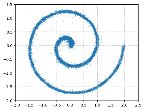
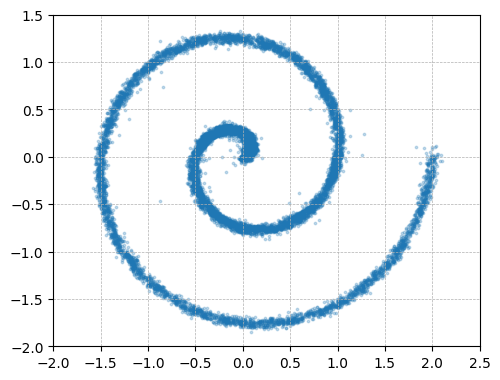
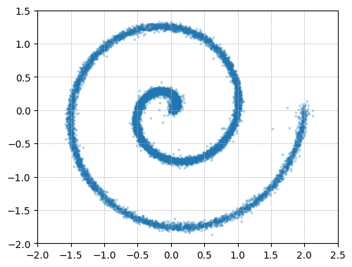
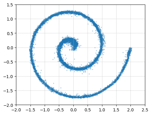
Think of an image as living on a narrow trail inside a huge forest. The forest represents all possible pixel combinations (very high‑dimensional space). The narrow trail is where real images “live” (a low‑dimensional manifold). Noise is like fog spread across the entire forest—it doesn’t stay on the trail.
Here’s how the authors set up their approach:
- Training task: They start with a clean image and add different amounts of noise to it. The model is trained to guess the clean image from the noisy one. This is called “x‑prediction.”
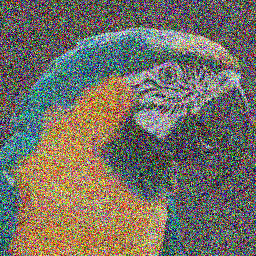
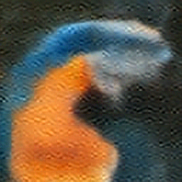
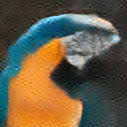
- Why x‑prediction: Because clean images live on a narrow trail, a limited‑capacity network can focus on that trail and ignore the fog. But if the model tries to predict noise (the fog itself), it needs to remember lots of details spread across the whole forest, which is much harder.
- Architecture: They use a plain Vision Transformer on large image patches (for example, 16×16 or 32×32 pixels per patch). Each patch becomes a “token” the Transformer processes.
- No extra tools: They avoid tokenizers, special pre-training, and add-on losses. It’s “Just image Transformers” (JiT).
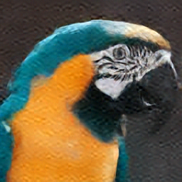
- Simple training and sampling: During training, the model predicts the clean image. For generation, they start from noise and repeatedly “denoise” using a standard numerical process, guiding the sample toward a clean image.
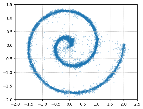
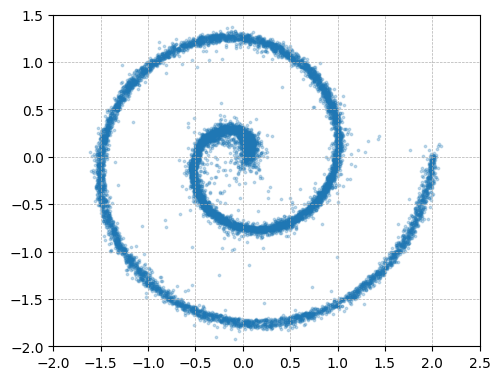
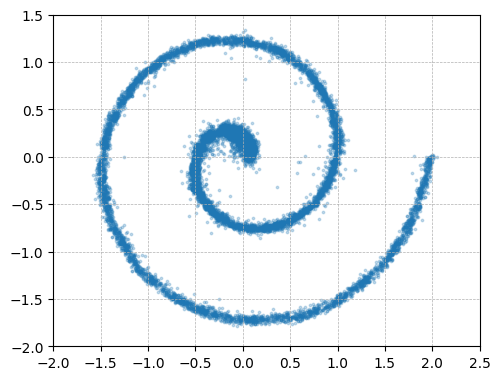
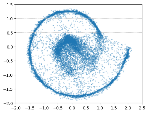
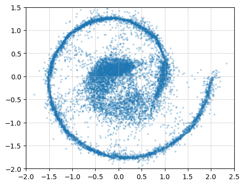
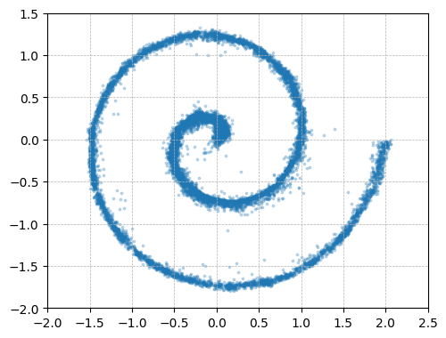
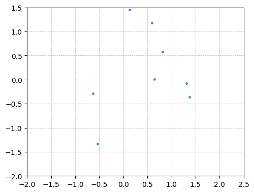
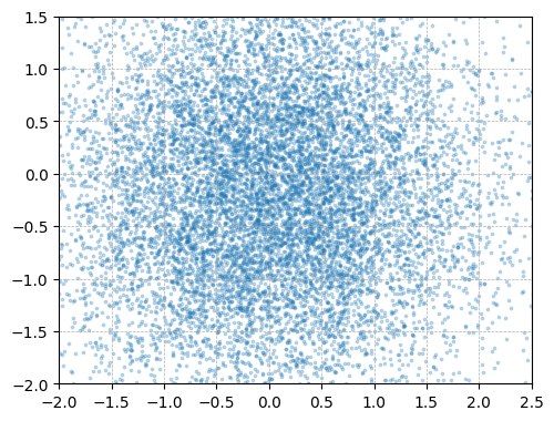
They also run a small “toy” experiment: hide a simple 2D pattern inside a much bigger space (like hiding a drawing inside a 512‑dimensional box). Only the clean‑image predictor recovers the pattern when the space gets very large; the noise or mixed predictions fail.
Main Findings
- Predicting the clean image works; predicting noise or a mixed “velocity” signal often fails when patches are high‑dimensional.
- Large patches are okay: Using patch sizes like 16×16 and 32×32 on ImageNet at resolutions 256, 512, and even 1024 works well with x‑prediction.
- Less can be more: The Transformer’s hidden width does not need to match the huge patch dimension. Surprisingly, adding a “bottleneck” (squeezing the patch down and then expanding it) can even improve results. This supports the idea that real images lie on a smaller, simpler structure.
- Tuning loss weights or increasing noise levels helps only if you are already predicting the clean image. These tricks cannot fix noise‑prediction at high dimensions.
- General-purpose upgrades to the Transformer (like better normalization or positional encoding) provide further gains without domain-specific hacks.
- Competitive results: Their “Just image Transformers” achieve strong scores on ImageNet without tokenizers, pre-training, or extra losses.
Why This Is Important
- Simplicity: It shows you don’t need complicated pipelines or pre-trained parts to get high-quality image generation from raw pixels.
- Scalability: The method scales to high resolutions and large patch sizes, which normally cause “catastrophic failure” for other setups that predict noise.
- Generality: Because it relies on standard Transformers and raw data, this approach could translate to other fields where designing tokenizers is hard, like proteins, molecules, or weather data.
- Back to basics: It brings diffusion models closer to their original idea—denoising—by actually predicting the clean image.
Implications and Impact
This work encourages researchers and engineers to rethink what diffusion models should predict. By focusing on the clean image, we can use simpler, more general models that handle very high‑dimensional inputs and still perform well. This “Diffusion + Transformer” approach, without domain-specific extras, may help the broader AI community build more robust, easy-to-transfer generators in many scientific and practical areas.
Knowledge Gaps
Knowledge gaps, limitations, and open questions
Below is a consolidated list of knowledge gaps, limitations, and open questions left unresolved by the paper that future work could address.
- Formal theory for why -prediction enables under-complete networks in high-dimensional spaces: derive capacity thresholds and error bounds that relate token dimensionality, network width, and training dynamics under manifold assumptions.
- Optimal bottleneck design: rigorously characterize when and why low-rank linear patch embeddings improve performance; determine the optimal bottleneck dimension as a function of resolution, dataset, and model size; test non-linear bottleneck embeddings.
- Generalization beyond ImageNet: validate -prediction with JiT on diverse datasets (e.g., CIFAR-10/100, LSUN, FFHQ, COCO) and across styles (natural, synthetic, medical), assessing robustness to data geometry and manifold quality.
- Other modalities: evaluate whether the self-contained “Diffusion + Transformer” paradigm with -prediction works for audio (waveforms/spectrograms), video, proteins, molecules, point clouds, and weather data; develop patch/tokenization strategies that avoid domain-specific tokenizers.
- Architecture dependence of the observed failure of -/v-prediction: test whether catastrophic failure persists for convolutional/U-Net models, hybrid ViT-conv architectures, or widened Transformers; isolate whether the failure stems from token dimensionality, attention, or conditioning.
- Noise schedule generality: the analysis claims applicability beyond linear schedules but experiments use linear , and logit-normal ; systematically compare cosine, EDM -parameterizations, variance-preserving schedules, and learned schedules for -prediction at high dimensionality.
- Full ablation of logit-normal parameters: only was varied; study the effect of , tails, truncation/clipping strategies, and schedule annealing on quality, stability, and training speed for -prediction.
- Handling the singularity near : the denominator in is clipped (default 0.05); quantify the bias introduced, its impact on convergence and sample quality, and whether reparameterizations can remove the need for ad hoc clipping.
- Sampling efficiency and speed: report and optimize the number of function evaluations (NFE), wall-clock sampling times, and quality–speed trade-offs; benchmark Euler vs Heun vs higher-order solvers, adaptive step sizes, and DDIM-like samplers tailored to -prediction.
- Training efficiency and resource footprint: provide measured training FLOPs, memory usage, throughput, and wall-clock times for 256/512/1024 settings; investigate gradient checkpointing, mixed precision, and sequence-length scaling strategies.
- Scaling laws: quantify empirical scaling laws for -prediction in JiT (FID vs parameters, data size, resolution, NFE), identify diminishing returns, and derive principled guidance for model and data scaling.
- Patch size and sequence length trade-offs: study variable and adaptive patch sizes, hierarchical or multi-scale patches, and their impact on spatial fidelity, boundary artifacts, and compute; clarify whether large patch sizes introduce subtle block artifacts.
- Positional encoding and attention design: the paper adopts RoPE and qk-norm; test robustness to alternative encodings (ALiBi, Rotary variants, relative positions) and attention mechanisms (local/windowed, cross-token convolutions) for large patch tokens.
- Conditioning mechanisms: beyond adaLN-Zero and in-context multiple class tokens, systematically ablate conditioning methods (FiLM, cross-attention, class embeddings) and the number/placement of conditioning tokens; characterize learned “in-context class token” behavior.
- Guidance dependence: quantify the reliance on classifier-free guidance (CFG) and CFG interval; measure FID/IS across guidance scales, and assess whether -prediction reduces or alters the need for guidance relative to -/v-prediction.
- Robustness to noise distribution: evaluate non-Gaussian, colored, or structured noise during training; test whether -prediction retains advantages when the corruption deviates from i.i.d. Gaussian assumptions.
- Precision–recall and diversity: complement FID/IS with precision/recall curves, KID, coverage metrics, and human evaluations to detect potential overfitting or mode collapse, especially at high resolutions and larger models.
- State-of-the-art comparisons: provide apples-to-apples comparisons against strong latent diffusion baselines (compute-, parameter-, and NFE-matched), including sample speed, memory use, and quality; clarify where pixel-space JiT is competitive or lagging.
- Integration with pretraining and auxiliary losses: while “self-contained,” systematically explore self-supervised pretraining (e.g., masked modeling), perceptual/adversarial losses, or representation alignment to quantify incremental gains for -prediction in high dimensions.
- ODE vs SDE training/sampling: -prediction is studied under flow/ODE; investigate stochastic formulations (SDE) and hybrid samplers to assess coverage and robustness, and whether the observed -/v-prediction failures persist under SDEs.
- Diagnosing -/v-prediction failures: develop targeted diagnostics (information retention across layers, token-wise mutual information, spectral bias) to pinpoint where and why high-dimensional noise/velocity prediction collapses.
- Intrinsic dimensionality and manifold verification: empirically measure intrinsic dimensionality of generated and real data patches; test whether JiT -prediction learns on-manifold projections (e.g., via local PCA, tangent estimation, geodesic distances).
- Stability and optimization: analyze training instabilities (loss spikes, exploding gradients) at high patch dimensionality; ablate optimizers, learning rates, weight decay, and normalization choices to identify stability regimes for -prediction.
- Multi-resolution and joint training: explore training a single JiT across multiple resolutions with shared weights or progressive resizing to improve efficiency and robustness.
- Domain-specific risks and biases: assess whether direct pixel modeling amplifies dataset biases or adversarial vulnerabilities; develop safety checks and mitigation strategies suitable for self-contained pixel-space diffusion.
Practical Applications
Overview
The paper introduces a simple but impactful shift in diffusion modeling: directly predicting clean data (x-prediction) instead of noise or mixed quantities (epsilon/v). Grounded in the manifold assumption, this enables effective modeling in very high-dimensional pixel spaces using plain Vision Transformers with large patches (“Just image Transformers”, JiT), without tokenizers, pre-training, or auxiliary losses. Key empirical findings include:
- x-prediction avoids catastrophic failures seen with epsilon/v-prediction at high per-token dimensionality.
- High-resolution pixel-space generation (256, 512, 1024) is feasible and compute-friendly by scaling patch size while keeping sequence length constant.
- Bottleneck embeddings can be beneficial, reducing dimensionality early with quality gains.
- The approach is self-contained and extensible with general Transformer advances (SwiGLU, RMSNorm, RoPE, qk-norm, in-context class tokens).
Below are practical applications, organized by time horizon, sector, and feasibility considerations.
Immediate Applications
These can be deployed now with modest engineering effort, using the paper’s training recipe (x-prediction + v-loss, logit-normal t-sampling, ODE solvers) and JiT architectures.
- Content creation and media (software/creative industries)
- Use case: Train compute-efficient, high-resolution (512–1024) pixel-space diffusion models for image generation without tokenizers or pre-training.
- Why it matters: Simplifies pipelines, reduces dependencies on proprietary encoders, and mitigates catastrophic failures at high resolutions.
- Tools/workflows: Drop-in x-prediction head in existing diffusion codebases; replace epsilon/v-loss with v-loss on x-pred outputs; scale patch size with resolution; adopt in-context class tokens and RoPE/qk-norm; Heun/Euler ODE sampling.
- Dependencies/assumptions: Availability of domain data; ImageNet-like benchmarks translate; sampling latency acceptable (or combined with standard acceleration techniques).
- Image restoration pipelines (healthcare imaging, photography, consumer devices)
- Use case: Denoising and artifact removal pipelines aligned with x-prediction (predict the clean image), improving stability at high resolution.
- Tools/workflows: Fine-tune JiT models on task-specific noise models; deploy bottleneck embeddings to shrink on-device footprints; maintain pixel-space to avoid tokenizer design.
- Dependencies/assumptions: Regulatory validation for medical use; real-world noise differs from synthetic Gaussian—requires calibration.
- Synthetic data generation for vision tasks (autonomous driving, retail, manufacturing)
- Use case: Produce diverse, high-res synthetic images to augment detection/segmentation training, with stable training in pixel space.
- Tools/workflows: Class-conditional JiT models; CFG interval; automated quality control using FID/KID plus task performance metrics.
- Dependencies/assumptions: Domain shift management; licensing/compliance for training data.
- Compute- and MLOps-friendly training for high-res diffusion (software infrastructure)
- Use case: Maintain constant sequence length across resolutions by scaling patch size (e.g., 16→32→64), enabling predictable compute and memory planning.
- Tools/workflows: Training orchestration templates that swap patch sizes with resolution; bottleneck-embedding “knobs” (e.g., 32–512) to tune throughput/quality.
- Dependencies/assumptions: GPU memory capacity for larger patches; stable AMP/mixed-precision training.
- Faster domain onboarding where tokenizers are hard to design (scientific imaging, satellite imagery)
- Use case: Build generative models on raw pixel data in domains lacking mature tokenizers (e.g., multispectral or hyperspectral images).
- Tools/workflows: JiT with minimal domain-specific changes; patch-wise preprocessing; x-pred v-loss training loop from the paper’s pseudo-code.
- Dependencies/assumptions: Noise model validation; proper calibration of t-schedules; labeled classes optional (in-context tokens improve conditioning when available).
- Open, legally simpler pipelines (policy/compliance)
- Use case: Reduce reliance on pre-trained encoders whose data provenance can be unclear.
- Tools/workflows: Self-contained training runs with documented datasets; reproducible recipe (noise schedule, loss, solver).
- Dependencies/assumptions: Still requires licensed training data; environmental impact of training should be tracked.
- Education and research baselines (academia)
- Use case: A clean, strong pixel-space baseline to study high-dimensional diffusion, manifold learning effects, and architecture scaling.
- Tools/workflows: Reproduce JiT-B/L/H/G at 256/512 with bottleneck studies; ablation libraries to toggle epsilon/v/x predictions and loss space.
- Dependencies/assumptions: Access to standard benchmarks (ImageNet) and compute.
Long-Term Applications
These require further research, scaling, or domain adaptation but are directly motivated by the paper’s findings and methodology.
- Multimodal and non-image domains with hard tokenization (biology, chemistry, weather, CFD)
- Use case: Generative modeling on raw continuous fields (protein density maps, molecular fields, geophysical grids) by predicting clean data directly in high-dimensional spaces.
- Potential products: “JiT-Fields” for weather nowcasting or climate downscaling; molecular field generators for drug discovery.
- Dependencies/assumptions: Confirm manifold structure and noise processes; appropriate patching schemes (spatiotemporal, multi-channel); rigorous validation vs baselines.
- 3D and 4D generative models (vision/graphics, robotics, AR/VR)
- Use case: Extend JiT to volumetric patches (voxels) or spatiotemporal patches for video/world models, leveraging x-pred’s stability in high dimensions.
- Potential products: Scene priors for NeRF-like systems; generative digital twins; robot world-model priors.
- Dependencies/assumptions: Efficient 3D patching and positional encodings; memory/runtime scaling; evaluation beyond FID.
- Medical imaging priors and reconstruction (healthcare)
- Use case: High-dim diffusion priors for MRI/CT denoising, under-sampled reconstruction, or dose reduction—favoring x-pred aligned with clinical targets.
- Potential products: Reconstruction aids integrated into scanners; post-processing denoisers with strong generalization.
- Dependencies/assumptions: Clinical validation and safety; domain shifts and non-Gaussian noise; regulatory approvals (FDA/CE).
- Energy and climate (energy, public sector)
- Use case: High-resolution generative downscaling of climate simulations or renewable resource maps using pixel-space JiT over gridded, multi-channel data.
- Potential products: Fast, high-fidelity scenario generators for planning and risk assessment.
- Dependencies/assumptions: Accurate multi-scale noise modeling; transparent uncertainty quantification; alignment with physical constraints.
- Finance and operations (finance, logistics)
- Use case: Denoising-style generative modeling of high-dimensional time–space signals (e.g., limit order book heatmaps, logistics demand fields) by predicting clean trajectories.
- Potential products: Synthetic scenario generators for stress testing; demand surface simulators.
- Dependencies/assumptions: Temporal extensions of JiT; non-Gaussian, heteroscedastic noise; strict risk controls and explainability.
- On-device, real-time generation and restoration (consumer hardware)
- Use case: Aggressive bottleneck embeddings and large-patch JiT to fit efficient generative models on future NPUs for live filters, denoise, and local editing.
- Potential products: Camera pipeline denoisers; privacy-preserving, local image editing assistants.
- Dependencies/assumptions: Hardware evolution; efficient few-step samplers; energy constraints.
- Standardization and governance (policy)
- Use case: Promote self-contained, reproducible diffusion training recipes that minimize opaque dependencies; encourage reporting of energy and data provenance.
- Potential outputs: Best-practice guidelines; auditing checklists for self-contained generative models.
- Dependencies/assumptions: Community and regulatory adoption; standardized benchmarks beyond FID.
- Accelerated sampling and distillation for JiT (software, academia)
- Use case: Develop few-step samplers and distillation tailored to x-pred in high-dimensional pixel space to achieve interactive latency.
- Potential tools: JiT-specific distillers; adaptive ODE solvers sensitive to patch dimension and t-schedules.
- Dependencies/assumptions: Research on stability/accuracy trade-offs; integration with CFG interval and guidance strategies.
- Text-conditional and multimodal extensions (software)
- Use case: Combine JiT’s pixel-space modeling with lightweight text encoders for caption- or prompt-conditioned generation, keeping the image side tokenizer-free.
- Potential products: Domain-specific promptable generators without autoencoders.
- Dependencies/assumptions: Language encoder selection reintroduces a pretrained component; alignment and safety filters.
Cross-cutting implementation notes
- Migration workflow from epsilon/v to x-pred:
- Replace network head to output x; compute v via algebraic transform; train with v-loss and a logit-normal t-sampler; clip 1/(1−t) denominator; consider CFG interval; adopt RoPE/qk-norm and in-context class tokens for quality boosts; test bottleneck embeddings (32–512).
- Risk/assumption checklist:
- Manifold assumption plausibility in target domain; noise model validity; compute and memory limits for large patches; dataset licensing; evaluation beyond FID (task metrics, human studies); regulatory/safety needs in sensitive domains.
In summary, by “letting denoising models denoise,” this work offers an immediately deployable recipe to stabilize and simplify high-dimensional diffusion in pixels, and a scalable foundation for broader scientific and industrial generative modeling where tokenization is costly or ill-posed.
Glossary
- adaLN-Zero: A conditioning technique that adapts layer normalization parameters to conditioning signals, initialized to zero to stabilize training. "We use adaLN-Zero \cite{Peebles2023} for conditioning"
- autoencoder: A neural network that learns to compress data into a latent representation and reconstruct it back, often used to learn low-dimensional manifolds. "Latent Diffusion Models (LDMs) \cite{Rombach2022} can be viewed as manifold learning in the first stage via an autoencoder, followed by diffusion in the second stage."
- BM3D: A classical image denoising algorithm that groups similar patches and performs collaborative filtering in a transform domain. "Classical methods, exemplified by BM3D \cite{dabov2007image} and others \cite{portilla2003image,elad2006image,zoran2011learning}, leveraged the assumptions of sparsity and low dimensionality to perform image denoising."
- bottleneck: An architectural constraint that reduces dimensionality to force compact representations, potentially improving generalization. "and surprisingly, a bottleneck design can even be beneficial, echoing observations from classical manifold learning."
- bottleneck linear embedding: A low-rank linear projection used to reduce and then expand patch dimensions before/after a Transformer, acting as a dimensionality bottleneck. "Bottleneck linear embedding."
- Classifier-Free Guidance (CFG): A sampling technique for conditional diffusion that guides generation without an explicit classifier by modulating conditional and unconditional scores. "with CFG \cite{ho2022classifier}"
- CFG interval: A schedule that varies guidance strength across sampling steps to improve quality and diversity. "with CFG interval \cite{kynkaanniemi2024applying}"
- curse of dimensionality: The phenomenon where high-dimensional spaces make learning and generalization difficult due to exponential volume growth and sparsity. "can still struggle to address the curse of dimensionality \cite{Chapelle2006SemiSupervised}."
- Denoising Autoencoders (DAEs): Models trained to reconstruct clean inputs from corrupted versions, leveraging the data manifold for representation learning. "Denoising Autoencoders (DAEs) \cite{vincent2008extracting,vincent2010stacked} were developed as an unsupervised representation learning method, using denoising as their training objective."
- Denoising Diffusion Probabilistic Models (DDPM): A diffusion framework that learns to reverse a noise-adding process by predicting noise or related quantities. "Denoising Diffusion Probabilistic Models (DDPM) \cite{Ho2020}: a pivotal discovery was to make noise the prediction target (i.e, $-prediction)." - **Diffusion Transformer (DiT)**: A Transformer architecture adapted for diffusion modeling, operating on tokens (e.g., image patches) with time conditioning. "Conceptually, this architecture amounts to the Diffusion Transformer (DiT) \cite{Peebles2023} directly applied to patches of pixels." - **Elucidated Diffusion Models (EDM)**: A formulation of diffusion around a denoiser with preconditioning to stabilize training and sampling. "EDM \cite{Karras2022edm} reformulated the diffusion problem around a denoiser function" - **Euler (method)**: A first-order numerical ODE solver used to integrate the reverse diffusion/flow dynamics. "Sampling step (Euler)" - **flow-based methods**: Generative models that learn continuous transformations (flows) from simple to complex distributions by integrating velocity fields. "diffusion models were connected to flow-based methods \cite{lipman2022flow,liu2022flow,albergo2023building}" - **Flow Matching**: A training objective that matches a learned velocity field to the true flow between noise and data distributions. "Flow Matching models \cite{lipman2022flow,liu2022flow,albergo2023building} can be interpreted as a form of $v$-prediction \cite{salimans2022progressive} within the diffusion modeling framework." - **flow velocity**: The time derivative of the interpolated sample along the diffusion/flow path, combining data and noise. "A flow velocity $vz$" - **Heun (method)**: A second-order ODE solver (improved Euler) commonly used to sample diffusion/flow models more accurately than Euler. "By default, we use a 50-step Heun." - **in-context class conditioning**: Providing class information as tokens within the Transformer sequence, enabling conditioning through context. "We also explore in-context class conditioning:" - **JiT (Just image Transformers)**: A minimalistic approach that applies plain Vision Transformers directly to image patches for diffusion without extra components. "Conceptually, our model is nothing more than ``Just image Transformers'', or JiT, as we call it, applied to diffusion." - **Latent Diffusion Models (LDMs)**: Diffusion models operating in a learned low-dimensional latent space instead of pixels to reduce computational cost. "Latent Diffusion Models (LDMs) \cite{Rombach2022} can be viewed as manifold learning in the first stage via an autoencoder, followed by diffusion in the second stage." - **latent tokenizer**: A module that encodes high-dimensional data (e.g., images) into a discrete or continuous latent representation for modeling. "no latent tokenizer \cite{Rombach2022" - **logit-normal distribution**: A distribution over a variable in (0,1) obtained by applying the logistic function to a normal variable; used to sample noise levels. "We use the logit-normal distribution over $t$ \cite{esser2024scaling}" - **manifold assumption**: The hypothesis that natural data lie near a low-dimensional manifold embedded in high-dimensional space. "The Manifold Assumption \cite{Chapelle2006SemiSupervised} hypothesizes that natural images lie on a low-dimensional manifold within the high-dimensional pixel space." - **manifold learning**: Techniques for learning low-dimensional, nonlinear representations that capture the intrinsic structure of data. "Manifold learning has been a classical field \cite{roweis2000nonlinear,tenenbaum2000global} focused on learning low-dimensional, nonlinear representations from observed data." - **NeRF**: Neural Radiance Fields; models that represent 3D scenes via neural networks rendering views from novel camera poses. "PixNerd \cite{wang2025pixnerd} adopts a NeRF head \cite{mildenhall2021nerf}" - **ordinary differential equation (ODE)**: A differential equation defining continuous-time dynamics; solved during sampling to generate data from noise. "sampling is done by solving an ordinary differential equation (ODE) for $zH{\times}W{\times}3H{\times}W{\times}128$ in the first layer)" - **patch embedding**: The linear projection that maps flattened image patches into token vectors for Transformer processing. "we turn the linear patch embedding layer into a low-rank linear layer" - **perceptual loss**: A loss computed in a feature space of a pretrained network to encourage perceptual similarity rather than pixel-wise accuracy. "no perceptual loss \cite{zhang2018unreasonable,Rombach2022}" - **pre-conditioned formulation**: A reparameterization of the model outputs/inputs to improve numerical stability and optimization in diffusion training. "EDM adopted a pre-conditioned formulation, where the direct output of the network is not the denoised image." - **qk-norm**: Query-key normalization in attention layers to stabilize training and improve scaling in Transformers. "SwiGLU \cite{shazeer2020glu}, RMSNorm \cite{zhang2019root}, RoPE \cite{su2024roformer}, qk-norm \cite{henry2020query}" - **representation alignment**: A training aid that aligns model representations to those from a pretrained model to improve learning. "no representation alignment \cite{repa}" - **RMSNorm**: Root Mean Square Layer Normalization; a normalization technique that normalizes activations using their RMS. "SwiGLU \cite{shazeer2020glu}, RMSNorm \cite{zhang2019root}, RoPE \cite{su2024roformer}, qk-norm \cite{henry2020query}" - **RoPE**: Rotary Positional Embeddings; a positional encoding method that introduces rotation to queries and keys for better extrapolation. "SwiGLU \cite{shazeer2020glu}, RMSNorm \cite{zhang2019root}, RoPE \cite{su2024roformer}, qk-norm \cite{henry2020query}" - **score-based diffusion models**: Generative models that learn the score (gradient of log-density) of noisy data distributions and sample via SDE/ODE integration. "closely related to modern score-based diffusion models \cite{Song2019,Song2021}" - **skip connections**: Direct links between network layers that help gradient flow and preserve information across scales. "accompanied by long-range skip connections." - **SwiGLU**: A gated activation function (Switch-GLU) improving Transformer feed-forward expressivity and training. "SwiGLU \cite{shazeer2020glu}, RMSNorm \cite{zhang2019root}, RoPE \cite{su2024roformer}, qk-norm \cite{henry2020query}" - **U-Net**: A convolutional encoder–decoder with skip connections widely used in pixel-space diffusion backbones. "most often a U-Net \cite{ronneberger2015u}" - **Vision Transformer (ViT)**: A Transformer architecture for images that processes non-overlapping patch tokens. "a plain Vision Transformer (ViT) \cite{Dosovitskiy2021}" - **v-prediction**: Predicting the flow velocity that combines data and noise within diffusion/flow formulations. "predicting the flow velocity (``\mbox{-prediction}'' \cite{salimans2022progressive})" - **x-prediction**: Predicting the clean data directly (e.g., the denoised image) instead of noise or velocity. "The formulation of -prediction is natural and not new" - **ε-prediction**: Predicting the additive noise (epsilon) that corrupted the data in diffusion training. "predicting the noise itself (known as ``$-prediction'')"
Collections
Sign up for free to add this paper to one or more collections.

