Skaling: Chinchilla's Exponents Meet Kaplan's Coupling
Abstract: Neural scaling laws are foundational for LLM development, yet standard formulations systematically under- and overestimate loss at data-scarce and overtraining extremes. This failure originates in the underlying assumption that model size and training data impact the loss independently. To address this, we introduce the Skaling law, a generalized functional form that couples model capacity and data through a single interaction exponent. This simple extension reduces the Mean Absolute Percentage Error (MAPE) by 1.5-3x across both interpolation and extrapolation regimes. When paired with a sparse grid strategy restricted to low-compute regimes, the Skaling law achieves accurate full-grid extrapolation using approximately 10x less compute than uniform sweeps. By enabling reliable performance prediction from small-scale experiments, the Skaling law provides a more robust and resource-efficient framework for allocating compute budgets in next-generation model training.

Paper Prompts
Sign up for free to create and run prompts on this paper.
Top Community Prompts
Explain it Like I'm 14
1. What is this paper about?
This paper studies how to predict the performance of LLMs without having to train many huge models.
Researchers usually measure a model’s loss, which is a number showing how often the model makes mistakes. Lower loss means better performance. Loss usually improves when:
- the model has more parameters—the adjustable numbers that give it more ability to learn;
- the model is trained on more tokens—pieces of text such as words or parts of words.
The paper argues that these two things do not work independently. A larger model may benefit differently from extra data than a smaller model does.
The authors introduce a new prediction formula called the Skaling law. It adds just one new feature to an older formula, allowing model size and training data to interact.
2. What questions did the researchers ask?
The main research questions were:
- Do model size and training data really affect loss independently?
- Can a simple formula that allows them to interact make better predictions?
- Can researchers use far fewer training experiments while still predicting the results of much larger experiments?
- Can the new formula help decide how much data a model should receive compared with its size?
These questions matter because training LLMs is extremely expensive. A better prediction method could prevent researchers from wasting enormous amounts of computing power.
3. How did they conduct the research?
Comparing different formulas
The researchers compared three ways of predicting loss:
- Chinchilla law: treats model size and training data as separate effects that are simply added together.
- Farseer law: uses many more adjustable parts to describe the relationship.
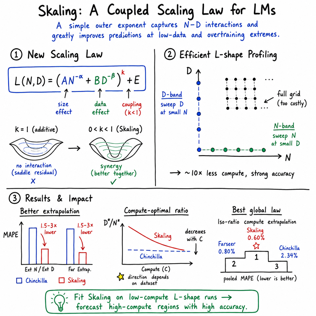
- Skaling law: keeps the simple structure of Chinchilla but adds one number, called the coupling exponent, to connect model size and data.
The Skaling formula is written roughly as:
Here:
- is the predicted loss;
- is model size;
- is the amount of training data;
- , , , and describe how loss changes;
- controls how strongly model size and data interact;
- represents a possible minimum loss that cannot be removed.
When , this becomes the older additive Chinchilla formula. When is different from 1, the two factors can influence each other.
Studying the “loss surface”
The researchers imagined the results as a landscape:
- one direction represents model size;
- another direction represents training data;
- the height represents loss.
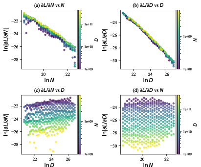
They used mathematical tools to study the slopes of this landscape. One tool, called moving least squares, is similar to estimating the shape of a hill by looking at nearby points. They also used a Gaussian process, which is a statistical method that estimates a smooth pattern from scattered data.
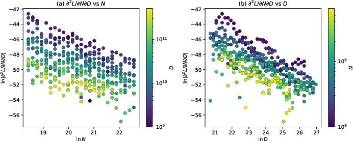
They especially examined the mixed derivative. In simple terms, this asks:
Does the benefit of making a model larger change depending on how much data it receives?
If the answer were no, the mixed derivative would be zero. The researchers found that it was not zero, suggesting that model size and data interact.
Testing on many model-training experiments
They tested the formulas on two collections of training runs:
- Farseer: 404 combinations of model sizes and data amounts;
- SK-Grid: 134 additional combinations created by the authors.
They tested both:
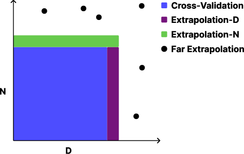
- interpolation: predicting results inside the range already studied;
- extrapolation: predicting results for larger models or more data than the experiments used.
They measured prediction error using MAPE, or mean absolute percentage error. For example, a MAPE of 2% means predictions were off by about 2% on average.
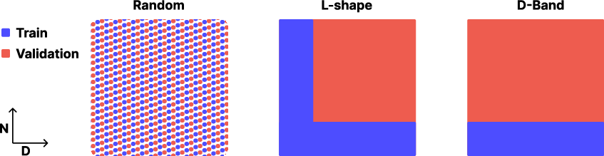
They also tested an L-shaped grid. Instead of training models across the entire size-and-data landscape, they trained:
- small models with different amounts of data;
- models of different sizes using a small, fixed amount of data.
This resembles measuring only two edges of a square rather than filling in every point.
4. What did they find?
The old formula made systematic mistakes at the edges
The Chinchilla formula often worked well for experiments in the middle of the tested range. However, it made larger errors in the corners, especially when:
- the model was very large but trained on little data; or
- the model was small but trained on a very large amount of data.
This happened because the formula assumed that model size and data acted independently.
Skaling usually predicted better
The Skaling law reduced prediction errors in most tests. On the full datasets, its errors were often between 1.5 and 3 times smaller than those of the Chinchilla law.
For example, on the SK-Grid data, the error for far extrapolation fell from:
- 5.17% with Chinchilla
- to 0.70% with Skaling
This is important because far extrapolation is similar to the real-world situation where researchers use small experiments to predict the behavior of much larger models.
The new method worked with about ten times less computing
The L-shaped strategy used about 10 times less training compute than a full grid.
Even with this much smaller amount of information, Skaling often remained as accurate as, or more accurate than, Chinchilla trained on the complete grid. For instance, on SK-Grid, far-extrapolation error was:
- 14.63% for Chinchilla using the L-shaped grid
- 1.15% for Skaling using the L-shaped grid
This shows that the new formula can make good use of carefully chosen small experiments.
More parameters were not automatically better
The Farseer formula had many more adjustable parameters, but it did not consistently perform better. In several tests, Skaling was more accurate.
This suggests that the important improvement was not simply adding complexity. Instead, Skaling used a structure that better matched the real relationship between model size and data.
The best data-to-model ratio can change with scale
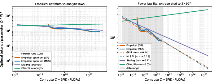
The paper also studied the best number of training tokens per model parameter. The authors found that the ideal ratio may change as models become larger.
However, the direction of this change was different in the two datasets. This means there is probably no single universal token-to-parameter rule that works for every model family and training setup.
5. Why are these findings important?
The research suggests that the common Chinchilla-style formula is too simple in some situations. It can look very accurate when tested only in the middle of a data range, while still making serious mistakes when predicting future, larger training runs.
The Skaling law offers three possible advantages:
- Better predictions: It more accurately estimates the loss of models trained with extreme combinations of size and data.
- Lower cost: Researchers may need roughly ten times less compute for early testing.
- Better planning: It may help laboratories decide how large a model should be and how much data it should use.
In everyday terms, the paper proposes a better map for planning a long journey. The old map worked well near familiar places but became unreliable at the edges. The new map adds one important detail—the way the two roads, model size and data, affect each other—so it can guide researchers more safely into unfamiliar territory.
The results do not mean that Skaling will work perfectly for every type of model or dataset. The authors found that the strength and direction of the interaction differed between experiments. Still, the method could make future language-model research more efficient, reducing the need for expensive trial and error.
Knowledge Gaps
The paper leaves the following knowledge gaps, limitations, and open questions unresolved:
- Limited external validation: The evaluation uses only two pretraining grids, including one proprietary/internal dataset (
Farseer) and one study-specific grid (SK-Grid); performance on independently collected datasets is not established. - Narrow architectural scope: It is unclear whether Skaling transfers across model families, transformer architectures, parameter-sharing schemes, tokenizer choices, sequence lengths, and training objectives.
- No validation on downstream capabilities: The experiments measure final validation loss only, so it remains unknown whether the coupling exponent improves scaling predictions for downstream accuracy, reasoning, retrieval, coding, or other task-specific metrics.
- Uncertain robustness to hyperparameter variation: All runs use prescribed near-optimal learning rates, batch sizes, and other settings; the law’s behavior under suboptimal or jointly optimized hyperparameters is not tested.
- Potential confounding from training prescriptions: The observed – interaction may partly reflect the StepLaw hyperparameter rules or other training-procedure choices rather than an intrinsic property of model capacity and data volume.
- Causal interpretation of coupling is unresolved: A nonzero estimated mixed derivative demonstrates empirical interaction, but it does not establish why the interaction occurs or whether it is caused by optimization, representation learning, memorization, data quality, or architecture.
- Sensitivity of mixed-derivative estimates is not fully quantified: The cross-derivatives depend on MLS neighborhood size, polynomial degree, weighting, regularization, grid density, and measurement noise; systematic sensitivity analyses and uncertainty intervals for these estimates are not reported.
- Independent confirmation of derivative findings is incomplete: Although a Gaussian-process estimator is described, the paper does not clearly report whether the principal mixed-derivative conclusions remain unchanged across GP kernels, length-scale choices, and alternative smoothing methods.
- Parameter identifiability remains weak: The fitted coupling exponent and irreducible loss trade off substantially, especially because the experiments do not reach the asymptotic saturation regime; the paper does not determine which parameter values are physically meaningful.
- The loss-floor interpretation is unresolved: The near-zero fitted on Farseer could represent parameter trade-off or model misspecification rather than a genuinely negligible irreducible loss floor.
- Functional-form selection is incomplete: Skaling is compared with Chinchilla and Farseer, but not with a broader set of alternatives, such as additive-plus-interaction models with monotonicity constraints, generalized means, spline surfaces, Gaussian processes, neural surrogate models, or other coupled power laws.
- The proposed one-parameter coupling may be dataset-specific: The fitted varies considerably across datasets and regimes, including values near the additive case; the conditions under which a single global is valid are not characterized.
- No hierarchical or transfer model is studied: The paper does not investigate whether coupling parameters can be shared across datasets or architectures while allowing dataset-specific amplitudes, floors, or exponents.
- Extrapolation distances are limited and irregular: The far-extrapolation sets contain only 7 Farseer points and 3 SK-Grid points, with different scale ranges and grid geometries, making reliability at substantially larger frontier scales uncertain.
- Long-horizon and very-large-model behavior is untested: The experiments do not establish whether the same functional form holds after much more training, at substantially larger parameter counts, or near data repetition and saturation limits.
- The claimed compute saving is design-dependent: The savings depend on the particular grid ranges, smallest model, shortest training horizon, and L-shape construction; the optimal sparse design under other budgets and scale ranges is not derived.
- The L-shape geometry is not optimized: The paper does not determine how many points should lie on each band, which anchor values should be selected, or how the design should adapt when the smallest model or shortest horizon is not sufficiently informative.
- Sparse-grid failure conditions are unknown: It is unclear how L-shape profiling performs when the observed grid does not include adequate boundary coverage, when measurements are noisy, or when the true interaction varies across the domain.
- Compute accounting may not generalize: The reported savings focus on training FLOPs and do not clearly include data preparation, evaluation, failed runs, hyperparameter searches, optimizer restarts, or engineering overhead.
- Optimal-allocation claims rely on restrictive assumptions: The closed-form compute-optimal ratio assumes a particular compute constraint and scaling form; effects from optimizer state, communication, memory, inference cost, architecture-dependent FLOP definitions, and fixed overheads are not considered.
- Predicted allocation trends are not validated at frontier scale: The reported 100-fold discrepancy and token-to-parameter recommendations are extrapolations; direct experiments comparing the competing allocation prescriptions at the claimed target scales are absent.
- The direction of allocation scaling remains unexplained: The sign of the optimal token-to-parameter trend differs between Farseer and SK-Grid, but the paper does not identify which dataset, architecture, or training factors determine that sign.
- Cross-validation uncertainty may be optimistic: The folds are drawn from the same underlying grids and are not independent experimental replications; uncertainty across random seeds, training runs, and datasets is not separated from fitting variability.
- Measurement noise is insufficiently characterized: The analysis uses final losses without reporting seed-to-seed variance, checkpoint variability, or correlations among runs sharing model sizes, data budgets, or training pipelines.
- MAPE may obscure practically important errors: Relative error on loss can overweight low-loss configurations and does not directly quantify errors in compute-optimal decisions, loss differences, or downstream utility.
- Baseline comparisons may not fully isolate functional-form effects: The more complex Farseer baseline may be disadvantaged by optimization difficulty, parameter bounds, or initialization; a systematically tuned likelihood or Bayesian comparison is not provided.
- Model misspecification is not tested statistically: The paper reports predictive metrics but does not provide likelihood-based comparisons, calibration tests, residual uncertainty estimates, or tests for systematic departures from the Skaling form.
- Interaction beyond one exponent is unexplored: The assumption that a single shared outer exponent captures all – interaction is not tested against models with scale-dependent or asymmetric coupling.
- Other scaling axes are left for future work: The applicability of Skaling to data quality, repeated data, sequence length, vocabulary size, sparsity, mixture-of-experts routing, modality, distillation, and data mixtures is asserted but not demonstrated.
- Practical deployment and online updating are unexamined: The paper does not show how the law should be updated as new runs arrive, how to detect when its assumptions fail, or how to incorporate uncertainty into real-time compute-budget decisions.
Practical Applications
Immediate Applications
- LLM pretraining budget planning — AI industry/software
- Replace or augment the additive Chinchilla law with the Skaling form when forecasting validation loss across model size and token budget .
- Use fitted parameters to estimate performance for candidate architectures and training horizons before committing to expensive runs.
- Workflow: train inexpensive boundary configurations, fit the five-parameter Skaling model, estimate loss across candidate pairs, and select the configuration with the best predicted loss under a fixed FLOP or monetary budget.
- Evidence: the paper reports approximately $1.5$– lower MAPE than Chinchilla in several interpolation and extrapolation settings.
- Dependencies: the target models must resemble the calibration runs in architecture, optimizer, sequence length, data quality, and training procedure. The law predicts loss, not downstream task accuracy, safety, latency, or serving cost directly.
- Low-cost scaling-law profiling — AI research labs and cloud providers
- Adopt the proposed L-shaped profiling grid: vary training tokens for small models in a D-band and vary model size at short training horizons in an N-band.
- Use this design to estimate scaling behavior with roughly an order of magnitude less profiling compute than dense full-grid sweeps.
- Potential product/tool: an experiment-planning module for platforms such as internal model-training systems or cloud ML services that automatically proposes low-compute trials and fits Skaling parameters.
- Dependencies: sufficient coverage of both axes is required; the smallest model and shortest-horizon runs must still exhibit informative scaling trends. The reported savings were demonstrated on two pretraining grids and may not transfer unchanged to other workloads.
- Frontier-run performance forecasting — large-scale model developers
- Fit Skaling using inexpensive runs and extrapolate to high-compute models along fixed token-to-parameter ratios or other operational training recipes.
- Use the predictions for go/no-go decisions, infrastructure reservations, checkpointing plans, and expected validation-loss targets.
- Evidence: on held-out high-compute Farseer runs, Skaling achieved a pooled MAPE of about , compared with for Chinchilla.
- Dependencies: extrapolation remains empirical rather than guaranteed. Performance can change under distribution shifts, new architectures, altered optimization schedules, deduplication, data contamination, or changes in the loss metric.
- Compute-optimal token-to-parameter allocation — AI infrastructure and model architecture
- Use the fitted Skaling parameters to calculate the compute-optimal ratio rather than assuming a universal ratio such as 20 tokens per parameter.
- Re-evaluate this ratio for each model family, data mixture, optimizer, and hardware-era training regime.
- Potential tool: a budget optimizer that jointly recommends parameter count, token count, training duration, and expected loss under a specified compute or energy budget.
- Dependencies: the paper shows that the direction of ratio change is dataset- and setup-specific: it decreases with scale on Farseer but increases on SK-Grid. The closed-form allocation therefore depends on reliable parameter fits and consistent compute accounting.
- Training-run experiment selection — academic machine-learning research
- Use mixed-derivative diagnostics, MLS, or Gaussian-process derivative estimates to test whether two scaling dimensions are genuinely separable.
- Before adopting an additive law, researchers can estimate and inspect whether boundary residuals show systematic saddle-shaped errors.
- Potential workflow: collect a modest pilot grid, estimate local gradients and cross-derivatives, compare additive and coupled models using held-out extrapolation—not only interpolation .
- Dependencies: numerical derivative estimates are sensitive to grid density, noise, neighborhood size, polynomial degree, kernel choice, and regularization. A nonzero estimate can also reflect measurement noise or optimizer instability.
- Model-training procurement and energy planning — cloud operations and sustainability
- Convert predicted loss improvements into more informed decisions about whether to purchase additional GPU time, extend training, increase model size, or acquire more data.
- Use the sparse profiling strategy to reduce the energy and carbon cost of preliminary scaling experiments.
- Dependencies: the paper measures training FLOPs, not full lifecycle energy or emissions. Real savings depend on hardware utilization, datacenter efficiency, communication overhead, and the cost of failed or repeated experiments.
- Internal model-development governance — industry and policy compliance
- Use uncertainty estimates from repeated cross-validation to attach confidence intervals to projected training outcomes and budget requests.
- Require extrapolation validation and sensitivity analysis before approving very large training runs.
- Dependencies: scaling-law error does not capture all operational risks, including data-rights issues, safety failures, security vulnerabilities, or deployment regressions. It should support, not replace, broader model-risk review.
Long-Term Applications
- Automated scaling-law services — AI platforms and MLOps
- Develop a reusable service that ingests training logs, validation losses, parameter counts, token counts, and FLOP estimates, then continuously refits Skaling and recommends the next experiments.
- Such a system could use active learning to select the most informative low-cost points, detect when the coupling exponent differs materially from $1$, and stop profiling when parameter uncertainty is sufficiently low.
- Dependencies: standardized logging and comparable loss measurements are necessary. Online fitting must account for changing data mixtures, curriculum schedules, optimizer settings, and model architectures.
- Multi-axis scaling laws — model research and scientific computing
- Extend the coupling idea beyond and to include sequence length, number of training epochs, data quality, repeated data, modality, sparsity, mixture-of-experts routing, context length, and inference-time computation.
- The resulting models could guide joint allocation among pretraining tokens, synthetic data, context length, model capacity, and post-training compute.
- Dependencies: adding axes may introduce parameter identifiability problems and require substantially more carefully designed experiments. A single coupling exponent may be insufficient when several interactions are strong.
- Scaling laws for downstream capability and reliability — healthcare, finance, education, and enterprise AI
- Calibrate coupled scaling models for task accuracy, calibration, factuality, robustness, latency, or domain-specific utility rather than validation loss alone.
- For example, a healthcare organization could estimate how model size and domain-specific tokens affect clinical extraction accuracy; a financial institution could forecast the benefit of additional training data under a fixed-risk or latency constraint.
- Dependencies: downstream metrics are often non-smooth, task-dependent, and affected by prompting, evaluation contamination, retrieval systems, and human workflows. Loss extrapolation should not be assumed to imply proportional gains in safety-critical performance.
- Data acquisition and curation optimization — data engineering and policy
- Combine Skaling with data-mixture scaling laws to decide whether additional budget should fund larger models, more tokens, higher-quality domain data, or improved deduplication.
- This could support procurement of licensed corpora, synthetic-data generation, multilingual expansion, and domain adaptation.
- Dependencies: the current experiments use controlled pretraining grids and do not establish how changes with data quality or mixture composition. Legal availability, privacy, licensing, and representativeness constraints may dominate the optimization.
- Adaptive compute allocation during training — autonomous ML systems
- Build training controllers that update the predicted loss surface as new checkpoints arrive and dynamically adjust the planned token budget, model expansion strategy, or early-stopping point.
- A system could compare the marginal value of additional parameters with the marginal value of additional data using the fitted gradients.
- Dependencies: the paper studies final validation loss for predefined runs, not online intervention. Dynamic resizing, optimizer-state transfer, catastrophic forgetting, and changing hardware availability require independent validation.
- Standardized benchmarking of extrapolation reliability — academia and public policy
- Establish benchmarks that evaluate scaling laws on interpolation, single-axis extrapolation, and far extrapolation, rather than reporting only in-grid fit quality.
- Public or inter-lab benchmark suites could help compare model-development forecasts and reduce wasteful replication of dense training grids.
- Dependencies: fair comparisons require consistent parameter counting, FLOP accounting, sequence lengths, data regimes, optimizer settings, and reporting of uncertainty. Results may vary substantially across datasets and architectures.
- Robotics and embodied AI resource planning — robotics
- Apply coupled scaling models to jointly predict the effects of policy-network size and interaction data, simulation steps, or robot trajectories.
- A robotics lab could use an L-shaped design to profile small policies across many trajectories and larger policies on short datasets before scaling to expensive real-world collection.
- Dependencies: the paper validates language-model pretraining loss, whereas robotics data are correlated, nonstationary, and costly to collect. Sim-to-real transfer and task success may not follow smooth power laws.
- Energy-system and scientific-model surrogate training — energy and scientific computing
- Use the methodology to plan the size of neural surrogates and the volume of simulation or sensor data needed for forecasting, optimization, or control.
- Sparse boundary experiments could reduce the cost of profiling large surrogate models for climate, materials, or power-grid simulations.
- Dependencies: domain losses may have multiple regimes, physical constraints, and distribution shifts. Monotonic improvement with model size and data—an explicit property of the Skaling form—may fail when overfitting or numerical instability occurs.
- Personalized learning and everyday AI services — education and consumer technology
- In principle, providers could estimate the tradeoff between model capacity and user-interaction data when designing tutoring, recommendation, translation, or on-device assistants.
- Coupled forecasts could inform whether to improve a model, collect more representative examples, or reduce compute for a deployment target.
- Dependencies: privacy, consent, fairness, feedback loops, and heterogeneous user behavior are central constraints. The paper provides no direct evidence that its pretraining-loss relationships apply to individual-level outcomes, so deployment would require extensive domain-specific studies.
Glossary
- Asymptotic behavior: The limiting behavior of a function as an input approaches infinity or another boundary. “Consider the asymptotic behavior of the loss function.”
- Autograd: Automatic differentiation software that computes derivatives of functions represented in code. “All scaling laws are fitted by minimizing a Huber loss in log space using L-BFGS-B with basin-hopping and autograd.”
- Basin-hopping: A global optimization method that searches for low-valued regions by repeatedly perturbing and locally optimizing candidate solutions. “All scaling laws are fitted by minimizing a Huber loss in log space using L-BFGS-B with basin-hopping and autograd.”
- Chinchilla law: An empirical scaling law that models reducible loss as additive power-law terms in model size and training data. “The widely used Chinchilla law~\citep{hoffmann2022training} decouples them completely.”
- Coefficient of determination: The statistic measuring the proportion of target variance explained by a fitted model. “the coefficient of determination () on the interpolation set only.”
- Concave: Describing a function whose rate of increase decreases, producing a downward-curving graph. “with the concave outer map makes the coupled reducible term decay more slowly at large scale”
- Compute-optimal allocation: The division of computational resources between model parameters and training data that minimizes predicted loss. “the Skaling law inherits Chinchilla's closed-form compute-optimal allocation”
- Cross-derivative: A derivative taken with respect to two different variables, measuring their interaction in a multivariable function. “For any , it reinstates a Kaplan-style coupling and a non-zero cross-derivative.”
- Cross-validation: A resampling procedure that repeatedly trains and evaluates a model on different data partitions. “To rigorously test the predictive capabilities and algorithmic stability of the fitted methods, we employ a comprehensive cross-validation framework.”
- Covariance matrix: A matrix describing pairwise statistical relationships among variables or observations. “where is the dense covariance matrix of the training inputs”
- Extrapolation: Prediction outside the range of values used to fit a model. “This approach allows us to explicitly quantify the uncertainty of our predictions, assess the variance of the fitted parameters, and test the models' ability to extrapolate reliably to unseen scales.”
- Farseer law: A more highly parameterized scaling-law formulation in which data-related parameters depend on model size. “The Farseer law~\citep{li2025predictable} makes the data exponent and amplitude depend on ”
- FLOPs: Floating-point operations, a measure of computational work. “with compute ranging from to FLOPs.”
- Gaussian process: A probabilistic model defining a distribution over functions, commonly used for regression and uncertainty estimation. “The global estimator fits a single Gaussian process to all points and differentiates its posterior mean in closed form.”
- Hessian matrix: A matrix of second-order partial derivatives that describes the local curvature of a function. “ is the Hessian matrix containing our target cross-derivative.”
- Huber loss: A robust loss function that behaves quadratically for small errors and linearly for large errors. “All scaling laws are fitted by minimizing a Huber loss in log space”
- Inductive bias: The preferences or assumptions a model’s structure imposes on the functions it can learn. “This suggests that the gain is not simply a consequence of adding parameters, but of using a functional form whose inductive bias matches the observed -- interaction.”
- Interpolation: Prediction within the range of values represented in the training data. “Validation (Interpolation): Randomly held-out points lying within the established boundaries of the training grid.”
- Irreducible loss: The component of prediction loss that cannot be reduced by increasing model size or training data. “alongside a free irreducible constant .”
- Iso-ratio slice: A subset of configurations sharing a constant ratio between two quantities, here training tokens and model parameters. “We group the runs into iso-ratio slices of constant token-to-parameter ratio ”
- Kernel: A function measuring similarity between input points, used by methods such as Gaussian processes. “In this work, we are using a Radial Basis Function (RBF) kernel with length-scale ”
- L-BFGS-B: A limited-memory quasi-Newton optimization algorithm that supports bound constraints. “using L-BFGS-B with basin-hopping and autograd.”
- L-shape sampling strategy: A sparse experimental design that samples points along two low-compute boundary bands of a parameter grid. “The mathematical structure of the scaling laws naturally motivates our primary approach: the L-shape sampling strategy”
- Marginal likelihood: The likelihood of observed data after integrating over a model’s latent or function values. “the GP explicitly models observation noise and automatically tunes its length-scales and noise levels by maximizing the marginal likelihood.”
- MAPE: Mean absolute percentage error, the average absolute prediction error expressed relative to the measured value. “the Skaling law reduces extrapolation MAPE by $1.5$-- relative to Chinchilla”
- Mesh-free: Not requiring data to lie on a regular mesh or grid. “we estimate using two mesh-free procedures”
- Mixed derivative: A derivative involving successive differentiation with respect to different variables. “The mixed derivative is the decisive test.”
- Monotonicity: The property of a function consistently increasing or decreasing as an input changes. “Skaling avoids this sign conflict because the interaction is in”
- Moving least squares (MLS): A local regression method that estimates a function or its derivatives by fitting weighted polynomials near each query point. “We probe the loss surface through its derivatives, estimated with the Moving least squares (MLS)”
- Power law: A relationship in which one quantity varies as a fixed power of another. “so the marginal derivatives decay approximately as power laws.”
- Posterior mean: The mean prediction of a probabilistic model after incorporating observed data. “The global estimator fits a single Gaussian process to all points and differentiates its posterior mean in closed form.”
- Predictive variance: A measure of uncertainty in a model’s prediction for a new input. “Additionally, the GP provides a closed-form predictive variance for this gradient”
- Radial Basis Function (RBF): A kernel whose value depends primarily on the distance between input points. “In this work, we are using a Radial Basis Function (RBF) kernel with length-scale ”
- Reducible loss: The component of loss that can be decreased through greater model capacity or more training data. “it removes the irreducible error and isolates the structure of the reducible loss.”
- Ridge regression: A regression method that adds an penalty to stabilize parameter estimation and reduce ill-conditioning. “by fitting this polynomial to the nearest neighbors using distance-weighted ridge regression”
- Saddle-shaped residual: A prediction-error pattern that changes sign across a surface in a shape resembling a saddle. “Chinchilla shows a saddle-shaped residual that grows toward the corners”
- Stationarity condition: An equation obtained by setting a derivative to zero, identifying a candidate optimum. “Minimizing the loss under a fixed budget reduces to the same stationarity condition as the additive Chinchilla law”
- Taylor expansion: A polynomial approximation of a function using its derivatives at a reference point. “This approach comes directly from Taylor expansion”
- Token-to-parameter ratio: The number of training tokens allocated per model parameter. “Frontier models such as DeepSeek~\cite{bi2024deepseek} typically lock in a fixed token-to-parameter ratio”
- Variance: A statistical measure of dispersion or uncertainty around an expected value. “Aggregating over folds, we report the mean of each metric together with its variance.”
Collections
Sign up for free to add this paper to one or more collections.

