On the origin of neural scaling laws: from random graphs to natural language
Abstract: Scaling laws have played a major role in the modern AI revolution, providing practitioners predictive power over how the model performance will improve with increasing data, compute, and number of model parameters. This has spurred an intense interest in the origin of neural scaling laws, with a common suggestion being that they arise from power law structure already present in the data. In this paper we study scaling laws for transformers trained to predict random walks (bigrams) on graphs with tunable complexity. We demonstrate that this simplified setting already gives rise to neural scaling laws even in the absence of power law structure in the data correlations. We further consider dialing down the complexity of natural language systematically, by training on sequences sampled from increasingly simplified generative LLMs, from 4,2,1-layer transformer LLMs down to language bigrams, revealing a monotonic evolution of the scaling exponents. Our results also include scaling laws obtained from training on random walks on random graphs drawn from Erdös-Renyi and scale-free Barabási-Albert ensembles. Finally, we revisit conventional scaling laws for language modeling, demonstrating that several essential results can be reproduced using 2 layer transformers with context length of 50, provide a critical analysis of various fits used in prior literature, demonstrate an alternative method for obtaining compute optimal curves as compared with current practice in published literature, and provide preliminary evidence that maximal update parameterization may be more parameter efficient than standard parameterization.
Paper Prompts
Sign up for free to create and run prompts on this paper using GPT-5.
Top Community Prompts
Explain it Like I'm 14
Plain-English Guide to “On the origin of neural scaling laws: from random graphs to natural language”
Overview (what the paper is about)
This paper tries to understand why bigger and better-trained AI LLMs get more accurate in such a predictable way. In many AI tasks, the error (how wrong the model is) drops following a simple pattern called a “power law” as you increase:
- the size of the model (number of parameters),
- the amount of data it sees,
- and the total compute (roughly, how much calculation you spend).
People have guessed that these neat patterns come from patterns already inside the data (like Zipf’s law in word frequencies). This paper tests that idea by building very simple, controllable “toy worlds” and showing that the same scaling patterns appear even when the data itself doesn’t have those power-law patterns. Then they gradually dial the data’s complexity up, from simple graph walks to real language, and watch how the scaling changes.
Key questions (what the authors wanted to find out)
- Do neural scaling laws appear even when the training data has no obvious power-law structure?
- How do the scaling rules change as we make the data more or less complex?
- What is the best way to measure and fit these scaling laws so we can plan training efficiently?
- Can simple models (like small, 2-layer transformers) already show the main scaling effects seen in big LLMs?
- Are there training setups (like a specific parameterization called “μP”) that use parameters more efficiently?
How they studied it (methods in everyday language)
The authors built a step-by-step ladder from very simple to more realistic data:
- Graph walks as simple “language”: Think of a graph as cities (nodes) connected by roads (edges). A “random walk” is like a traveler who starts in some city and repeatedly chooses a random road to take next. If you write down the sequence of visited cities, it looks like a sequence of tokens (like words). Predicting the “next city” from the current one is just like predicting the next word from the previous word. In language modeling, predicting based on the last one word is called a “bigram” model.
- Different graph types:
- Erdős–Rényi graphs: random connections, no power-law patterns in node connections.
- Barabási–Albert graphs: “scale-free” graphs where a few nodes have many connections (a power-law pattern).
- They also tried “biased” walks where some paths are more likely, to gently introduce power-law-like structure.
- Dialing complexity toward real language: 1) Language bigrams (pairs of tokens) learned from a real dataset. 2) Text generated by tiny transformers trained on real data (1-, 2-, and 4-layer generators), which captures more structure than bigrams but is still simpler than true language. 3) Real natural language.
- Measuring learning curves:
- you increase model size (N),
- you increase data size (D),
- or you optimize the mix of both for a fixed compute budget.
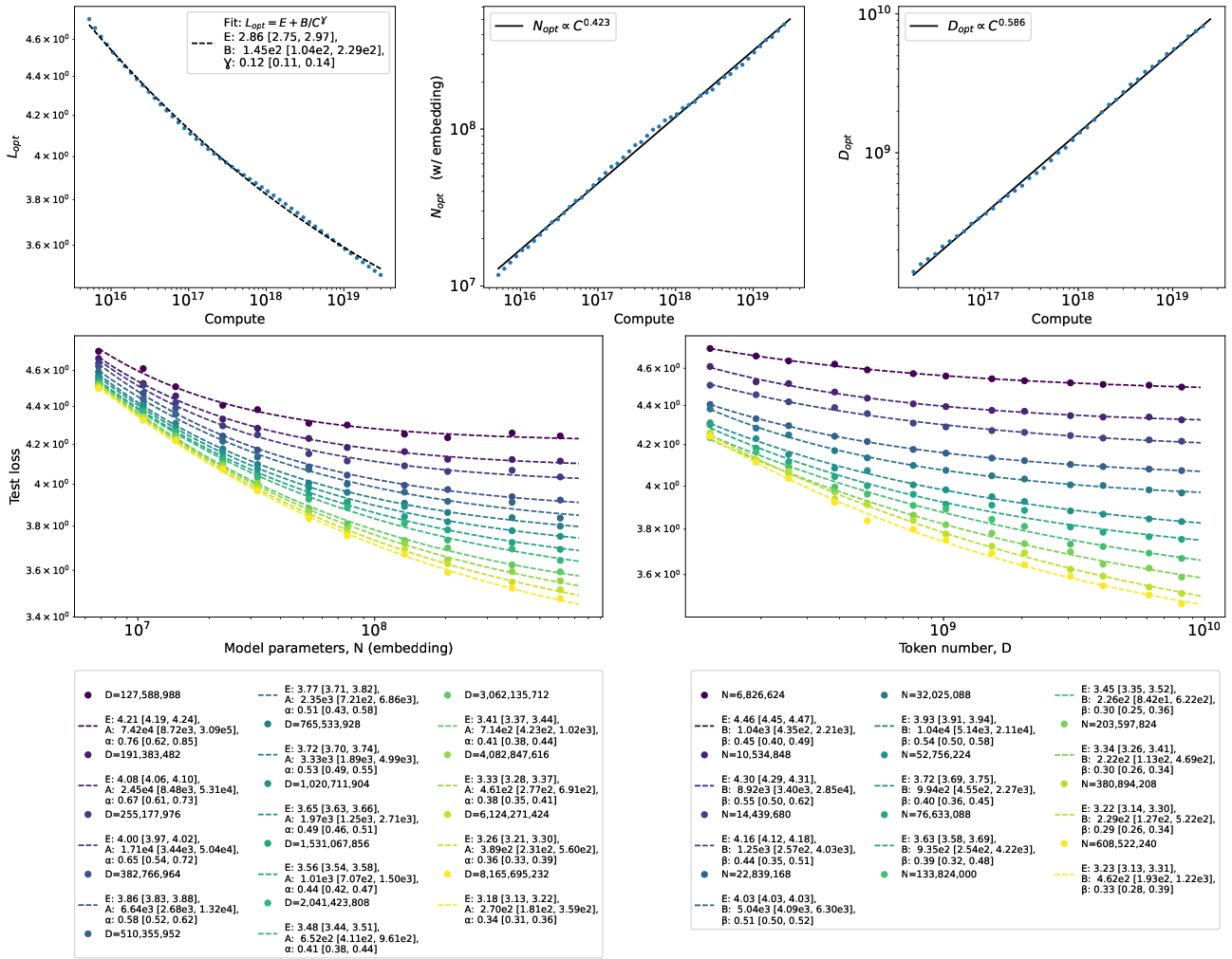
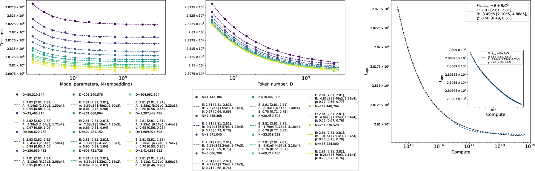
A simple, widely used fit for these curves is:
- L is the loss (error).
- E is the “irreducible loss” (like the part you can’t beat because the task has some inherent uncertainty).
- The exponents α and β tell you how quickly things improve with more parameters or more data. Bigger exponents mean faster improvement.
- Fitting the curves carefully:
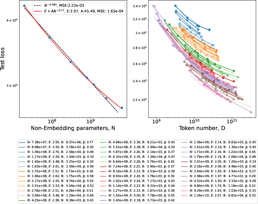
- They show it’s crucial to include the “irreducible loss” E when fitting. If you drop it, you can badly underestimate how fast models improve.
- They compare different fitting methods and argue that a common 2D formula (“Chinchilla fit”) is less accurate than using standard ML regression (like a small neural network) to map (N, D) → loss. This matters if you want reliable “compute-optimal” plans—how best to spend a fixed budget across model size and data.
Main findings (what they discovered and why it matters)
Here are the essential takeaways:
- Scaling laws show up even with “no-power-law” data
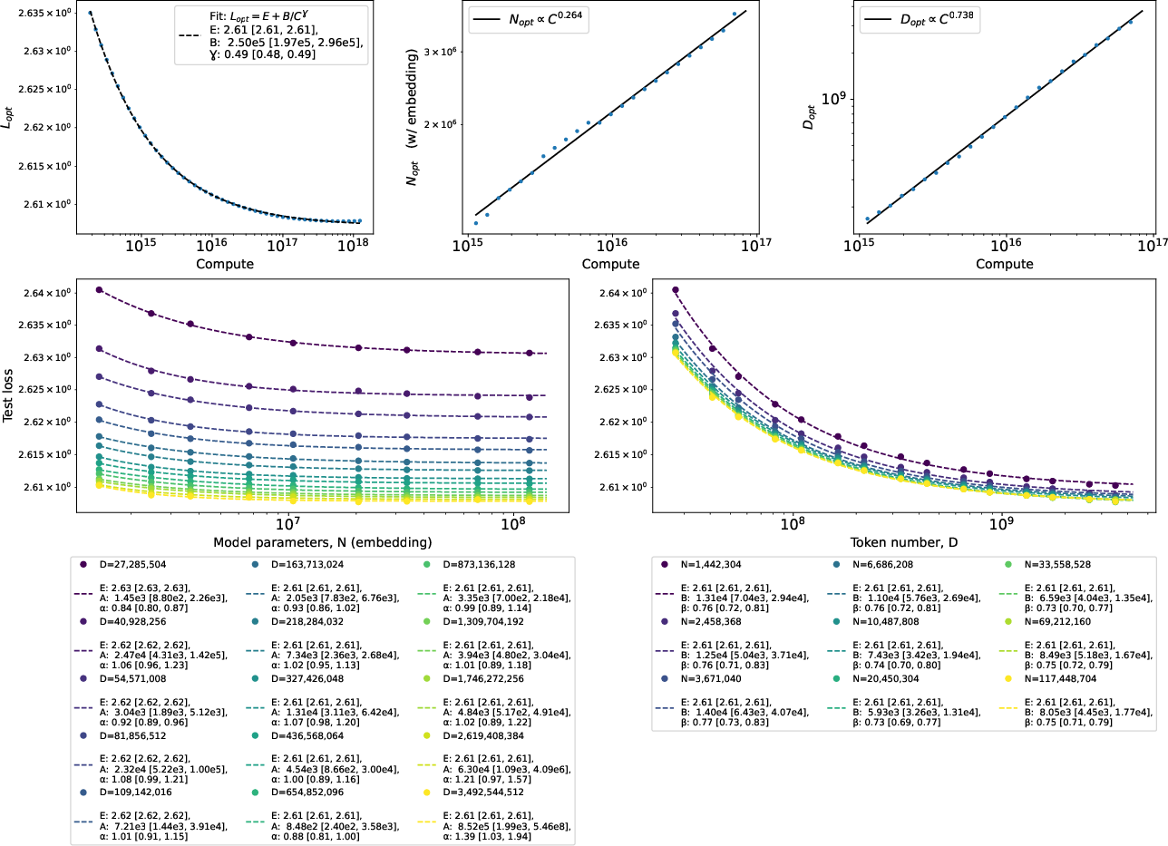
- Training transformers to predict random walks on simple random graphs (Erdős–Rényi), where the data has no built-in power-law patterns, still produced clean power-law learning curves.
- Why this matters: It suggests that the neat scaling behavior is not only a property of the data; it also comes from the learning setup (architecture + objective + optimization). That’s a big clue about the deeper “why” behind scaling laws.
- As data gets more structured, scaling exponents change in a smooth, sensible way
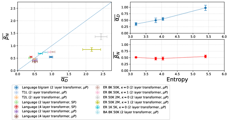
- They “dial up” data complexity: language bigrams → text from tiny transformers (T1L, T2L, T4L) → real language.
- One of the key exponents (roughly, the one tied to data size, β) stays fairly stable (around one-half), while the exponent tied to model size or data complexity changes in a monotonic way. In plain terms: the “shape” of improvement changes gradually and predictably as the data becomes richer.
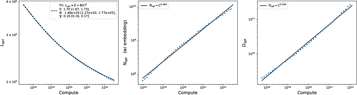
- Simple models can reproduce big, famous results
- Using tiny 2-layer transformers with short context windows (like 100 tokens), they recover several well-known scaling behaviors from earlier large-scale studies. Even differences between famous results (like OpenAI’s Kaplan et al. vs. DeepMind’s Chinchilla rules) can be explained partly by whether you count “embedding” parameters (the big tables that map tokens to vectors) in the model size. This means you don’t always need huge, expensive experiments to study scaling—small, careful ones can teach a lot.
- Better fitting = better planning
- They argue that:
- You must include the irreducible loss E in fits, or you’ll underestimate how quickly models can improve.
- A popular 2D formula (the “Chinchilla” fit) often fits the data worse than standard ML regression. Using a small neural net to fit loss as a function of (N, D) can give more accurate predictions for “compute-optimal” training plans (how to split your budget between model size and data size).
- Why this matters: Better fits mean better decisions when spending time and money on training.
- A training setup called μP may be more parameter-efficient
- “Maximal Update Parameterization” (μP) is a way to set a model’s internal scaling so different sizes train more consistently. The authors see early signs that μP might get more out of each parameter than standard setups, which could shift the “best” way to allocate compute.
Why this is important (implications and impact)
- Understanding the roots of scaling laws helps us predict the future of AI progress. If we know why and how error drops with more data and compute, we can plan smarter training runs and save huge amounts of resources.
- The fact that scaling laws appear even without power-law patterns in the data means these laws are more universal than we thought. They likely come from how transformers learn sequences with the cross-entropy objective, not only from quirks in natural data.
- The “dial up the complexity” approach gives a controlled playground to test theories. Researchers can run cheap experiments on synthetic data (like graph walks) and still learn lessons that apply to real language.
- Better fitting tools (including keeping the irreducible loss term and using standard ML regression) can make compute planning more reliable across labs and projects.
- If μP is more parameter-efficient, future models could be trained more economically, reaching the same accuracy with fewer parameters.
In short: The paper shows that neural scaling laws are robust, not just a coincidence of natural data. It offers clearer measurement tools, cheaper testing grounds, and hints for more efficient training—all of which can speed up and stabilize progress in building smarter LLMs.
Knowledge Gaps
Knowledge gaps, limitations, and open questions
The paper leaves several concrete questions and limitations that future work could address:
- Formal mechanism: No theoretical explanation is provided for why transformers trained with cross-entropy on Markov sequences exhibit power-law loss scaling even when the data lacks power-law correlations; what optimization dynamics, architectural properties, or capacity/variance trade-offs set the exponents?
- Exponent attribution: The study does not map scaling exponents to measurable dataset or graph properties (e.g., spectral gap, mixing time, degree heterogeneity, stationary entropy, rank–frequency slope); can α, β, γ be predicted from such statistics?
- Limited graph ensembles: Experiments focus on ER and BA graphs with mostly unbiased, stationary walks; directed graphs, weighted graphs with structured community/hierarchy, hypergraphs, and higher-order n-grams (n>2) are unexplored.
- Incomplete sweep of correlation strength: The biased-walk parameter κ is only tested at 0 and 1; a continuous sweep of κ is needed to quantify how exponents and fit quality evolve with the heaviness of the transition probability tail.
- Scale limitations: Results are predominantly with 2-layer transformers and short contexts (50–100) at modest N and D; do the same conclusions hold at scales typical of state-of-the-art LLM pretraining (longer context windows, deeper models, larger parameter counts and datasets)?
- TnL dataset fidelity: The “Transformer-generated n-layer (TnL)” synthetic datasets are assumed to interpolate complexity toward natural language, but their closeness to real language (distributional properties, long-range dependencies) is not validated; how do TnL statistics (entropy, mutual information, memory length) compare to real corpora?
- Complexity measure: Dataset “complexity” is proxied by the irreducible loss E from 1d fits; this is a loose lower bound and may be biased by limited N/D; develop robust complexity metrics (e.g., conditional entropy at varying orders, mutual information decay, long-range correlation measures) and relate them quantitatively to the scaling exponents.
- Long-range dependencies: Random walks (bigram-equivalents) have short memory and exponential autocorrelation; how do scaling laws change in datasets with controlled long-range dependencies (e.g., higher-order n-grams, hierarchical grammars, synthetic processes with power-law memory)?
- Bigram truncation and smoothing: The language bigram model removes rare bigrams (≤5 occurrences), altering tail behavior; assess how rare-event truncation and smoothing choices (e.g., Kneser–Ney, additive smoothing) affect scaling exponents and fit quality.
- Architecture breadth: Only decoder-only GPT-style models are studied; head count, width/depth trade-offs, positional encodings, normalization schemes, residual scaling, and attention variants are not ablated; how do these architectural choices shift scaling exponents and compute-optimal policies?
- Loss/objective scope: Experiments use cross-entropy next-token loss; do scaling laws and exponents persist under other objectives (MSE, contrastive pretraining, sequence-level losses), finetuning regimes, or RLHF?
- Training regime: One-epoch training (C≈6ND) is assumed; early stopping, multi-epoch data reuse, curriculum schedules, and optimizer settings (and their interaction with compute accounting) are not explored; how do these change optimal a, b, γ?
- Embedding parameter inclusion: The reconciliation of Kaplan vs. Chinchilla through embedding inclusion is shown only in shallow models; quantify systematically across depths/context lengths whether embedding accounting is the dominant factor and how other factors (learning-rate schedules, optimizer, weight decay) contribute.
- muP parameterization: Evidence that maximal-update parameterization (muP) is more parameter-efficient is preliminary; a comprehensive, multi-scale comparison (varying depth, width, context, datasets) is needed to establish tokens-per-parameter compute-optimal laws under muP and their robustness.
- Fit methodology and uncertainty: While 1d power-law fits outperform exponentials, other plausible forms (stretched exponentials, broken power laws, log-polynomial corrections) are not evaluated; provide principled model selection, uncertainty quantification for exponents, and assess potential regime changes (piecewise scaling).
- 2d regression extrapolation risk: Compute-optimal curves derived via neural-network regression lack interpretability and theoretical guarantees; evaluate extrapolation sensitivity, compare with Gaussian process or spline-based nonparametric regressors, and propagate uncertainty into a, b, γ estimates.
- Spectral links: The relationship between the transition matrix spectrum (eigenvalue gap, tail distribution) and learned scaling exponents is hypothesized but not tested; design graph ensembles with controlled spectra to directly test exponent dependence on spectral properties.
- Domain generality: Only language data and graph walks are studied; test whether “scaling without data power laws” generalizes to other domains (vision, audio, code, mathematics) and whether exponents differ systematically by modality.
- Capability-level validation: The study focuses on token-level loss; examine whether scaling exponents translate consistently into downstream capability scaling (QA, reasoning, long-context tasks), especially in settings with short memory versus long dependencies.
- Hyperparameter robustness: Exponent estimates are based on limited hyperparameter sweeps and a fixed set of schedules; quantify sensitivity to learning rate, batch size, weight decay, optimizer, and initialization across datasets and architectures.
- Reproducibility and seeds: The stability of exponents across random seeds and runs is not reported; provide multi-seed variance and confidence intervals for fitted scaling exponents and compute-optimal parameters.
- Compute accounting: The FLOPs model C≈6ND ignores overheads and hardware/precision effects; calibrate actual compute and training time across settings and assess sensitivity of compute-optimal conclusions to realistic cost models.
- Directed vs. undirected walks: Language bigrams correspond to directed transitions; many graph experiments use undirected unbiased walks; systematically compare scaling exponents between directed and undirected settings to align with language modeling more closely.
- Data diversity: Fineweb-edu and GPT-2 tokenization are used; investigate sensitivity of exponents to corpus composition (web vs. books), tokenization schemes (BPE vs. unigram), and data quality filtering.
- Depth discrimination: T4L sequences produce nearly identical exponents to T2L for a 2-layer learner; test whether deeper learners can distinguish T2L vs. T4L and whether the scaling exponents reflect the generator’s depth or compositional hierarchy.
Practical Applications
Immediate Applications
The following are actionable use cases that can be deployed now, organized by sector. Each item notes key assumptions or dependencies that affect feasibility.
Industry
- Compute-optimal training planning for LLMs
- Use one-dimensional loss fits with irreducible loss terms and neural-network regression to predict compute-optimal curves and choose N and D for a fixed budget.
- Potential tools/products: “Compute-Optimal Planner” (a small internal service to fit L(N,D) and output N_opt, D_opt), “Scaling Dashboard” (MLOps integration to track loss curves and exponents).
- Workflows: run a small grid of training runs (vary N, D), fit using 1D power laws and NN regression, derive N_opt/D_opt, decide whether to include embeddings in N for reporting, then launch full-scale training.
- Assumptions/dependencies: consistency of optimizer and training schedule across the grid; reliable estimation of irreducible loss E; data/architecture held fixed during extrapolation.
- Low-compute A/B evaluation of optimizers and architectures
- Reproduce key language-model scaling-law results with 2-layer transformers and short context lengths (≈100) to compare algorithmic changes before committing to high compute.
- Potential tools/products: “Shallow-LLM Eval Harness” that standardizes 2-layer tests with fixed context length and batch sizes.
- Assumptions/dependencies: correlation between shallow-model scaling behavior and deeper models; same loss metric (cross-entropy); consistent tokenization.
- Tunable-complexity synthetic benchmarks for sequence modeling
- Use random walks on Erdős–Rényi and Barabási–Albert graphs and transformer-generated language (TnL) sequences to benchmark scaling behavior and training stability without expensive real corpora.
- Potential tools/products: “GraphWalkBench” (dataset generator + reference tasks), “ComplexityDial” (pipeline to generate T1L/T2L/T4L and bigram datasets).
- Assumptions/dependencies: synthetic tasks capture salient scaling dynamics of real pretraining; graph parameters and walk biases are controllable and well documented.
- Parameter-efficiency gains via maximal update parameterization (μP)
- Adopt μP to potentially reduce parameters for a given performance envelope and revisit token-per-parameter heuristics.
- Workflows: compare μP vs. standard parameterization on small grids, then deploy μP broadly if confirmed.
- Assumptions/dependencies: preliminary evidence holds across tasks/data; optimizer and LR schedules are compatible; adequate internal validation.
- Reporting and comparability standards for scaling experiments
- Include irreducible loss (E) in all fits; disclose whether embedding parameters are counted in N; avoid defaulting to the 2D Chinchilla fit when NN/kernel regression fits yield lower MSE.
- Potential tools/products: “ScalingFit” library (1D fits with E, NN/kernel regression, bootstrap CI).
- Assumptions/dependencies: organizational alignment on metrics; access to fitting tooling and CI pipelines.
- Energy and cost forecasting for training runs
- Use improved compute-optimal predictions (C ≈ 6ND) to forecast energy draw and cost for different N/D mixes and training durations.
- Assumptions/dependencies: stable FLOP/machine efficiency estimates; known data throughput; consistent epoch policy (often 1-epoch in the paper).
Academia
- Experimental platforms to study origins of scaling laws
- Leverage tunable-complexity sequences (graph walks, TnL, bigrams) to bridge theory (linear/kernel models with MSE) and practice (auto-regressive models with cross-entropy).
- Assumptions/dependencies: shared datasets and code; reproducible fitting procedures (including offsets and bootstrap CIs).
- Teaching modules on scaling phenomena
- Course labs using random walks and shallow transformers to demonstrate how scaling laws emerge even without power-law data correlations.
- Assumptions/dependencies: modest compute resources (1013–1016 FLOPs); accessible open-source tokenizers/transformers.
- Methodological improvements for fitting loss curves
- Replace 2D parametric formulas with neural/kernel regression to fit L(N,D) and use 1D fits with irreducible loss for interpretable exponents.
- Assumptions/dependencies: agreed-upon evaluation splits and error metrics; careful handling of outliers and hyperparameter sweeps.
Policy
- Evidence-based compute governance and transparency
- Require reporting of compute-optimal planning, irreducible loss fits, and whether embeddings are included in parameter counts to standardize disclosures and comparability.
- Assumptions/dependencies: community consensus on reporting templates; regulator familiarity with scaling-law terminology.
- Practical reproducibility with low compute
- Promote shallow-model baselines (2-layer, short context) for independent verification of scaling behavior before large-scale pretraining investments.
- Assumptions/dependencies: availability of open datasets (e.g., Fineweb-edu subsets) and reference code.
Daily Life
- Cost-effective open-source model development
- Community projects can use shallow transformers and synthetic benchmarks to validate methods before scaling, reducing compute costs and environmental impact.
- Assumptions/dependencies: accessible tooling; coordination on shared baselines and tokenizers.
- Education and skill-building
- Hobbyist-friendly labs that explore sequence modeling with graphs and bigrams to understand LLM training fundamentals and scaling effects.
- Assumptions/dependencies: curated tutorials; modest GPU availability.
Long-Term Applications
These use cases likely require further research, scaling, or development before broad deployment.
Industry
- Automated curriculum learning that dials dataset complexity
- Dynamic training pipelines that start with synthetic graph walks or bigrams, then progress to TnL and natural language to optimize scaling exponents and training efficiency.
- Potential tools/products: “CurriculumDialer” (complexity-aware data scheduler), “ExponentTracker” (online estimation of α, β, γ).
- Assumptions/dependencies: validated links between dataset entropy/structure and exponents; robust online fitting; stable model behavior under curriculum shifts.
- Architecture and optimizer design targeting exponent improvements
- Systematically search for changes that increase α and β, improving asymptotic efficiency of deep learning methods.
- Assumptions/dependencies: reliable small-scale proxies for large-scale exponents; automated search infrastructure.
- Enterprise compute marketplaces informed by scaling predictions
- Procurement platforms that allocate compute budgets based on predicted returns from L(N,D) fits, including parameterization choice (μP vs. standard).
- Assumptions/dependencies: integration with cloud/cluster schedulers; contractual energy/cost models.
Academia
- Unified theory connecting sequence modeling with cross-entropy to observed power-law loss scaling
- Formal frameworks that explain exponents without relying on power-law data correlations, using graph/hypergraph sequence processes.
- Assumptions/dependencies: new mathematical tools; collaboration across theory and empirical groups.
- Reasoning benchmarks via graph walks and hypergraphs
- Stepwise inference and chain-of-thought tasks grounded in controllable graphical structures to study scaling of reasoning capabilities.
- Assumptions/dependencies: benchmark standardization; agreement on evaluation metrics beyond perplexity.
Policy
- Standards and audits for compute-optimal training
- Policies that require ex-ante scaling-law projections (with irreducible loss) and track deviation against actual results to manage energy use and environmental impact.
- Assumptions/dependencies: accepted audit methodologies; data access for regulators.
- Funding and risk assessment frameworks
- Public or philanthropic funding models that evaluate proposals using low-compute scaling proxies to estimate likely gains from large-scale pretraining.
- Assumptions/dependencies: refined proxy-to-large-scale correlation; robust peer review processes.
Daily Life
- Consumer-facing AI features trained with complexity-aware curricula
- Applications (assistants, educational tutors) trained with staged data complexity to lower costs while preserving performance quality.
- Assumptions/dependencies: transferability from synthetic pretraining to end-user tasks; productization pipelines.
- Education platforms for scalable AI literacy
- Interactive tools where learners can tune graph parameters and observe how scaling exponents change, building intuition about model and data design.
- Assumptions/dependencies: funded platform development; accessible compute.
Notes on Assumptions and Dependencies
- Most fits assume 1-epoch training, cross-entropy loss, and consistent tokenization; deviations can change observed exponents.
- Including vs. excluding embedding parameters in N materially affects compute-optimal N/D splits and comparability across studies.
- μP appears promising for parameter efficiency, but evidence is preliminary; confirm across diverse tasks and scales before broad adoption.
- Synthetic benchmarks (graph walks, TnL) should be validated as proxies for real-language scaling when used to guide expensive training decisions.
- Reliable estimates of irreducible loss (E) are critical; omitting E can severely understate exponents and mislead planning.
- Outlier handling, bootstrap confidence intervals, and reporting of fit quality (MSE, Huber loss) are necessary for credible extrapolation.
Glossary
The following is an alphabetical list of advanced domain-specific terms from the paper, each with a brief definition and a verbatim usage example from the text.
- Adjacency matrix: A square matrix representing which nodes in a graph are connected by edges. Example: "The spectrum of the adjacency matrix obeys a semicircle law, which is typical of random symmetric matrices."
- Auto-regressive sequence modeling: A modeling setup where the next element in a sequence is predicted based on previous elements. Example: "The above theories based on linear models with mean square error (MSE) loss are rather far from the setting of auto-regressive sequence modeling with cross-entropy loss."
- Barabási-Albert ensemble: A family of graphs generated via preferential attachment that produces scale-free degree distributions. Example: "Our results also include scaling laws obtained from training on random walks on random graphs drawn from Erdös-Renyi and scale-free Barabási-Albert ensembles."
- Barabási-Albert preferential attachment model: A graph-generation mechanism where new nodes attach preferentially to high-degree nodes, yielding a power-law degree distribution. Example: "One way to construct a scale-free graph is via the Barabási-Albert preferential attachment model \citep{barabasi1999emergence}, which gives ."
- Bias-corrected and accelerated bootstrap method: A statistical resampling technique providing improved confidence interval accuracy (BCa bootstrap). Example: "Brackets indicate 95\% confidence intervals obtained from bias-corrected and accelerated bootstrap method (see Appendix \ref{app:fitting} for details)."
- Bigram graph: A graph representation where nodes are tokens and directed edge weights encode bigram probabilities. Example: "In the case of a bigram model (), this defines a directed, weighted graph, which we refer to as the bigram graph."
- Bigram model: An n-gram LLM with n=2 that conditions each token on the previous one. Example: "In the case of a bigram model (), this defines a directed, weighted graph, which we refer to as the bigram graph."
- Broken power law: A distribution that follows different power-law exponents over different ranges. Example: "Language results are from Fineweb-edu using GPT-2 tokenizer; unigram distribution is a standard Zipf plot, while bigram distribution shows broken power law."
- Chain of thought reasoning: Multi-step reasoning where intermediate steps are explicit, akin to traversing a path in a graph. Example: "walks on graphs can be used to model stepwise inference and chain of thought reasoning \citep{khona2024understandingstepwiseinferencetransformers,Besta_2024}."
- Chinchilla formula (2d): A two-parameter family used to fit test loss as a function of model size and data size. Example: "which we refer to as the 2d Chinchilla formula."
- Compute optimal curves: Curves describing the best achievable loss as a function of fixed computational budget by optimally choosing model and data sizes. Example: "demonstrate an alternative method for obtaining compute optimal curves as compared with current practice in published literature"
- Compute optimal scaling laws: Relationships describing how optimal loss and optimal choices of parameters/data scale with compute. Example: "demonstrate a simple neural network regression method to obtaining compute optimal scaling laws, which is different from methods presented in the literature to date"
- Cross-entropy loss: A loss function measuring the divergence between predicted and true categorical distributions; standard in language modeling. Example: "auto-regressive sequence modeling with cross-entropy loss."
- Decoder-only GPT-style transformer: A transformer architecture that predicts the next token using only a causal (decoder) stack. Example: "We use a decoder-only GPT-style transformer to perform next-token prediction."
- Directed, weighted hypergraph: A generalization of graphs where edges (hyperedges) can connect more than two nodes and have direction and weights. Example: "In that case, the -gram model defines a directed, weighted hypergraph with nodes."
- Erdös-Renyi graph: A random graph model where each possible edge is included independently with a fixed probability. Example: "The simplest class of random graphs are Erdös-Renyi graphs."
- FLOPs (floating point operations): A measure of computational cost counting arithmetic operations. Example: "The compute in FLOPs (floating point operations) can be expressed exactly in terms of , , and number of training steps"
- Huber loss: A robust loss function less sensitive to outliers, combining quadratic and linear behaviors. Example: "fit using a Huber loss () as in \citep{hoffmann2022training}"
- Hyperparameter sweep: Systematic exploration over hyperparameter configurations to find optimal settings. Example: "L(N,D) is taken to be the optimal loss over a hyperparameter sweep:"
- Irreducible loss: The asymptotic floor of the loss due to intrinsic uncertainty/entropy in the target distribution. Example: "Dropping the constants (referred to as the irreducible loss) in the 1d fits"
- Kernel regression: A nonparametric method for function approximation using kernel-weighted averages. Example: "Many theoretical works have shown that in linear or kernel regression, power laws in the test loss do in fact originate from power laws in the data"
- Markov random walk: A sequence generation process moving between nodes with transition probabilities depending only on the current state. Example: "The simplest non-trivial generative model of sequences is a Markov random walk on a graph."
- Maximal update parameterization (μP): A model parameterization scheme intended to stabilize training dynamics across scales. Example: "We also show preliminary results that maximal update parameterization \citep{yang2021tensor} might be more parameter-efficient than standard parameterization"
- Mean square error (MSE) loss: A regression loss equal to the average squared difference between predictions and targets. Example: "The above theories based on linear models with mean square error (MSE) loss are rather far from the setting of auto-regressive sequence modeling with cross-entropy loss."
- Preferential attachment: A mechanism where new nodes are more likely to connect to high-degree nodes, producing power-law degree distributions. Example: "One way to construct a scale-free graph is via the Barabási-Albert preferential attachment model \citep{barabasi1999emergence}, which gives ."
- Random walk, unbiased: A walk on a graph where transition probabilities depend only on uniform edge choices (or degree-normalized for undirected graphs). Example: "An unbiased random walk on an undirected graph has the transition probability $p(u|v) = \frac{A_{uv}{\text{deg}(v)}$"
- Scale-free graph: A graph whose degree distribution follows a power law, meaning many low-degree nodes and a few hubs. Example: "A scale-free graph \citep{barabasi1999emergence} is defined such that a randomly chosen node has degree with probability for large , with ."
- Semicircle law: A result from random matrix theory where eigenvalue distributions follow a semicircle density. Example: "The spectrum of the adjacency matrix obeys a semicircle law, which is typical of random symmetric matrices."
- Small-world graph: A graph with high clustering and short average path lengths compared to random graphs. Example: "Co-occurrence matrices from natural language corpora in particular have been shown to determine a scale-free, small-world graph"
- Spectral gap: The difference between the largest and second-largest eigenvalues of a transition matrix; controls mixing rates. Example: "Recall that random walks have an exponentially decaying auto-correlation, with the time-scale for the exponential decay set by the spectral gap of the transition matrix."
- Stationary distribution: A probability distribution over states that remains unchanged by the transition dynamics of a Markov chain. Example: "The stationary distribution is "
- Stationary joint distribution: The stationary probability distribution over tuples of consecutive states for higher-order Markov processes. Example: "The initial nodes can be chosen from the stationary joint distribution on nodes."
- Transition matrix: A matrix where entry (i,j) gives the probability of transitioning from state j to i; governs Markov dynamics. Example: "Recall that random walks have an exponentially decaying auto-correlation, with the time-scale for the exponential decay set by the spectral gap of the transition matrix."
- Transformer-generated n-layer (TnL) datasets: Synthetic text datasets produced by sampling from trained transformers with n layers. Example: "we refer to these datasets as Transformer-generated -layer (TnL) datasets."
- Tunable complexity: A property of datasets or tasks where structural difficulty can be systematically increased or decreased. Example: "would be to study sequence modeling with datasets of \it tunable complexity\rm,"
- Unigram distribution: The marginal distribution over individual tokens (single-word frequencies). Example: "Sampling from a bigram model corresponds to sampling a random walk on the bigram graph, with transition probabilities , where is the stationary distribution on nodes, and equivalently the unigram distribution of the sequence."
- Variance-limited regime: A scaling regime where performance improvements are limited by estimation variance rather than bias. Example: "Note that this can be thought of as the \"variance-limited\" regime for power law scaling of data in the language of \citep{bahri2021explaining}."
- Zipf plot: A rank-frequency plot used to visualize Zipf-like distributions. Example: "Language results are from Fineweb-edu using GPT-2 tokenizer; unigram distribution is a standard Zipf plot, while bigram distribution shows broken power law."
- Zipf's law: An empirical law stating that word frequencies in natural language are inversely proportional to their rank. Example: "it is well-known that the frequency of words in a corpus of text follows Zipf's law"
- Two-dimensional parametric fits: Functional forms that model loss as a joint function of model and data sizes with a small set of parameters. Example: "It is common to consider two-dimensional parametric fits of the form \citep{hoffmann2022training,bhagia2025establishingtaskscalinglaws, muennighoff2023scaling,gadre2024overtraining,zhang2024map,kang2025demystifyingsyntheticdatallm}"
Collections
Sign up for free to add this paper to one or more collections.

