How to Allocate Your Tokens? Scaling Laws with Training Steps and Batch Size
Abstract: We propose a scaling law that takes into account model size and training data while explicitly splitting the latter into training steps and batch size (called three-term law). Fitting the proposed law on a large set of training runs, we find that it correctly recovers the scaling of the optimal batch size. Moreover, because it makes use of training runs with suboptimal batch size, our proposed law can be robustly fit with a significantly smaller amount of training runs. We further show that the three-term law can be used to derive scaling laws for suboptimal batch sizes, and that it matches previous empirical findings related to the critical batch size.
Paper Prompts
Sign up for free to create and run prompts on this paper using GPT-5.
Top Community Prompts
Explain it Like I'm 14
How to Allocate Your Tokens? Scaling Laws with Training Steps and Batch Size — A Simple Guide
What is this paper about?
This paper is about finding a smart way to train large AI LLMs (like chatbots) using a fixed amount of text, called “tokens.” It asks: if you have a certain number of tokens to train with, how should you split them between:
- how many examples you show the model at once (the batch size), and
- how many times you update the model (the number of training steps), so that you get the best results?
The authors propose a simple formula—called a “scaling law”—that predicts how performance changes as you vary model size, batch size, and training steps. Then they test whether this formula matches real training behavior.
What questions are the authors trying to answer?
In easy terms, the paper tackles four main questions:
- Can we build a single, simple rule that explains how model performance depends on:
- model size ( = how big the model is),
- batch size ( = how many tokens per step), and
- training steps ( = how many updates)?
- If we only know our total token budget (), what is the best batch size to use?
- Can we learn this rule without running lots of expensive training experiments (saving time, money, and energy)?
- If we can’t use the best batch size (because of hardware limits), how much performance do we lose—and what range of “pretty good” batch sizes still wastes little compute?
How did they study this? (Methods in everyday language)
Think of training a model like baking lots of cookies:
- Model size = how big your oven is.
- Total tokens = how much dough you have (total ingredients).
- Batch size = how many cookies you bake at once (trays in the oven).
- Steps = how many rounds you bake.
You can split your dough into larger batches (big , fewer rounds ) or smaller batches (small , more rounds ), as long as (total cookies baked stays the same).
The authors propose a simple performance formula:
- Loss (lower is better) = E + A/Nα + B/Mβ + C/Kγ
In symbols:
- With (your fixed token budget)
What this means:
- Bigger models help ( up ⇒ loss down).
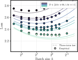
- Larger batch size helps—but only to a point ( up ⇒ loss down).
- More training steps help—but also with diminishing returns ( up ⇒ loss down).
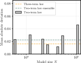
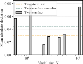
They tested this formula using two large collections of real training runs (“Li” and “OpenEuroLLM”), where many models were trained with different sizes, token budgets, and batch sizes. They compared two approaches:
- A “three-term law” (one shared formula across all model sizes: depends on , , ).
- A “two-term law” (one formula per model size: depends on , only).
They also tried training with only a few batch sizes per setup to see if they could still discover the right rule—this simulates saving compute in practice.
Finally, they studied a real-world idea called the “critical batch size”: the point beyond which increasing batch size no longer speeds up training much.
What did they find, and why does it matter?
Here are the main takeaways:
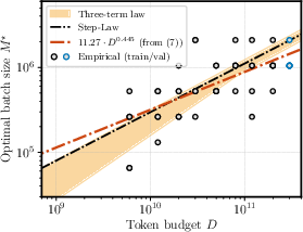
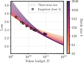
- The new three-term formula works and gives a clear rule for the best batch size.
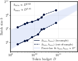
- If total tokens are , the best batch size grows roughly like .
- Importantly, the best batch size does not depend on model size —it mainly depends on how many total tokens you plan to use.
- This matches earlier studies, but here it naturally falls out of a single formula that also predicts the final loss.
- You don’t need tons of expensive experiments to learn this rule.
- Using the three-term formula, the authors could get almost the same best-batch-size rule using only two batch sizes per setup.
- That cut the number of required training runs to about 28% of the full set. That’s a big compute and energy savings.
- The formula also helps when you can’t use the best batch size.
- Hardware might force you to use smaller or larger batches.
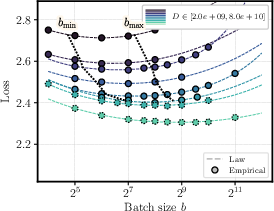
- The authors show a two-stage method to estimate a “good enough” range of batch sizes that wastes at most about 5% extra compute.
- As a rough rule of thumb, the acceptable range is fairly wide—often spanning about a 4× range in batch size—so you have flexibility.
- It matches how “critical batch size” behaves in practice.
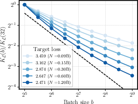
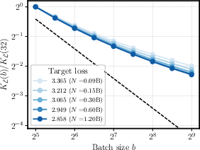
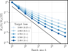
- The number of steps needed to reach a target quality flattens out after some batch size (increasing batch size stops helping much).
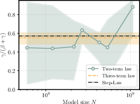
- Their formula reproduces a key pattern observed in practice: this flattening depends mostly on the total token budget , not on the model size .
- This is helpful guidance: using the biggest possible batch size is not always a good idea.
- A caution when reducing back to the classic two-term law (model size + data only).
- If you convert their three-term law back to the classic form , the implied “compute-optimal” model size and data split can differ from what you’d get if you fit that classic form directly.
- Translation: if you’re planning billion-token, billion-parameter runs, the exact formula you choose can change your recommended plan. So, pick carefully.
Why is this important?
- It gives practical, easy-to-use rules for planning large model training:
- How big should your batches be?
- How many steps should you run?
- What happens if you can’t use the ideal batch size?
- It can save a lot of compute, time, money, and energy by reducing the number of training runs needed to discover good settings.
- It aligns with real-world behavior (like critical batch size), so it’s more trustworthy in practice.
Final thoughts and future impact
This work helps teams train big LLMs more efficiently by:
- Providing a simple, unified rule that links model size, batch size, and steps.
- Showing how to choose near-optimal batch sizes even under hardware constraints.
- Reducing the cost of finding good settings.
There are still open questions. The formula assumes the learning rate is already well tuned, and results may vary with different optimizers or training tricks. Future work could extend the formula to include the learning rate or account for different optimizers.
Still, if you’re planning a big training run, this paper gives you a clearer, cheaper roadmap for how to split your token budget between batch size and steps—and that can make a real difference.
Knowledge Gaps
Knowledge gaps, limitations, and open questions
Below is a concise, concrete list of unresolved issues that the paper identifies or implies, phrased to guide follow‑up research.
- External validity across setups
- Validate the three-term law on additional domains (e.g., vision, speech, protein modeling), architectures (e.g., MoE, recurrent, transformer variants), and training regimes (instruction tuning, RLHF, multi-task) to assess generality beyond dense LLM pretraining.
- Systematically test robustness across tokenizers, vocabulary sizes, and data distributions (quality/mixture/curriculum/duplication), given the law depends only on token count and not data quality.
- Sensitivity to optimizer and schedule
- Extend the law to explicitly include optimizer and schedule parameters (e.g., learning rate magnitude and schedule, AdamW , weight decay, EMA, gradient clipping, Muon), and re‑fit on controlled ablations to quantify how shift with optimizer choices.
- Determine whether the independence of from persists with different optimizers or schedules (cosine, constant, linear, one-cycle) and across noise‑scale regimes.
- Learning rate modeling
- Incorporate learning rate as an explicit variable into the law (including schedule shape), leveraging theoretical bounds (e.g., links to noise scale and KL conditions) to jointly model and reduce the need for separate LR sweeps.
- Quantify the minimal LR sweep required to fit the extended law within specified error bars.
- Suboptimal batch-size prediction limits
- The three-term law underfits loss at suboptimal ; the two‑stage fix assumes . Test and report when this assumption breaks, and develop a principled single‑stage model that predicts suboptimal performance without relying on .
- Determine the minimum sweep density in (and placement strategy) needed to estimate the ‑suboptimal interval to a target error.
- Additive separability assumption
- The law assumes additive separability in and terms (). Probe for interaction effects (e.g., cross‑terms like or multiplicative couplings) by fitting alternative forms and conducting likelihood‑ratio/model‑selection tests.
- Critical batch size validation
- Empirically measure (steps to reach a fixed target loss) under controlled settings and compare directly to the law’s predictions rather than deriving from fitted parameters, to validate claimed invariances to and dependencies on .
- Clarify the relationship between the law’s and the empirically observed “critical batch size” across optimizers, schedules, and weight decay settings.
- Chinchilla reduction mismatch
- The reduction of the three-term law to a Chinchilla‑type law yields different implied than a direct Chinchilla fit. Diagnose the source (e.g., underfitting, parameter identifiability, misspecification) and develop fitting procedures or priors that reconcile the two.
- Provide uncertainty intervals for the implied compute‑optimal to quantify decision risk in deployment.
- Parameter identifiability and uncertainty
- Analyze identifiability of and establish conditions under which these parameters are recoverable from partial sweeps; report parameter confidence intervals and correlations.
- Study the sample complexity of fitting: how many configurations are needed for stable recovery of and within prescribed error tolerance?
- Irreducible loss term
- The fitted on the Li dataset is inconsistent with nonzero entropy of language. Investigate regularization constraints, hierarchical priors, or multi-task calibration to obtain realistic and decouple it from finite‑compute effects.
- Sequence length and effective batch
- The law uses but does not model explicitly beyond this product. Test whether and scale consistently when varying (long‑context training, context packing), and determine if additional ‑dependent terms are needed.
- Data scaling beyond token count
- Augment the model to incorporate data quality/novelty/duplication (e.g., effective tokens or diversity metrics) rather than raw alone, and quantify shifts in under such controls.
- Breakdown regimes and piecewise behavior
- Identify regimes where power‑law behavior in or breaks (very small , extremely large , severe gradient accumulation) and fit piecewise or saturating forms; specify thresholds where the current law ceases to hold.
- Hardware and wall‑clock considerations
- Translate “5% compute waste” into wall‑clock and throughput terms under realistic hardware constraints (communication, memory/activation offloading, kernel efficiency) to provide actionable batch‑size intervals for practitioners.
- Reproducibility and dataset access
- Some analyses rely on OpenEuroLLM (not public at writing). Release data and scripts, and re‑run fits to confirm conclusions and parameter stability post‑release.
- Theoretical grounding
- Provide rigorous conditions under which the exponents and additive structure arise from optimization theory (beyond relaxing $1/2$ to free exponents), and connect constants to measurable quantities (e.g., gradient noise scale, curvature, Lipschitz/PL/KŁ constants).
- Derive when and why should be independent of , and characterize counterexamples.
- Metric choice and downstream validity
- The law targets final test cross‑entropy/perplexity. Evaluate whether the same scaling holds for downstream task performance, calibration, and emergent abilities; if not, propose task‑conditioned extensions.
- Compute model assumptions
- The compute proxy omits optimizer costs, activation recomputation, parallelization overhead, or memory‑bound effects. Calibrate the law with more realistic compute models and quantify the impact on and recommendations.
- Smoothing and evaluation protocol
- Assess how loss smoothing, early stopping, and evaluation frequency influence fits; standardize an evaluation protocol to reduce fit variance across datasets.
- Extension to regularization effects
- Incorporate weight decay and other regularizers (label smoothing, dropout) into the law, building on prior links between weight decay and batch size, to improve predictions of both and .
Practical Applications
Immediate Applications
The following items summarize practical, deployable uses of the paper’s three-term scaling law and associated procedures that can be adopted now across industry, academia, policy, and daily practice.
- Training planning and cost reduction for LLMs and other deep models (software/AI, cloud)
- Use the three-term law
L(N, M, K) = E + A/N^α + B/M^β + C/K^γto select near-optimal batch size and number of steps under a fixed token budget , without requiring full batch-size sweeps. - Workflow: For each , run 2–3 batch sizes, fit the law, and infer and ; this reduces runs to ~28% of a full sweep while matching prior optimal batch-size scaling.
- Tools/products: A “Batch Size Advisor” plugin for
PyTorch LightningorHuggingFace Trainerthat logs , fits the three-term law on-the-fly, and recommends the next configuration; integration withRay Tunefor guided hyperparameter search. - Assumptions/dependencies: Uses AdamW-like training with stable LR schedules; requires small sets of runs per ; law parameters are dataset/setup dependent; sequence length affects constants.
- Use the three-term law
- Resource-aware MLOps scheduling and GPU utilization (cloud, enterprise ML)
- Allocate GPU memory and throughput by selecting batch sizes within the -suboptimal interval that wastes ≤5% compute.
- Workflow: Apply the paper’s two-stage fit (per , fit a simplified curve, then generalize ) to set practical batch-size bounds respecting compute and memory limits.
- Tools/products:
ThreeTermFitlibrary to estimate (N, D)DK_{\bar{L}}(b)\bar{L}K_{\bar{L}}(b)bb(N, D)M^\starE(N, M, K)\epsilonb\epsilon[b_{\min}, b_{\max}]DbMKDKMDD\epsilonM^\star(D)K_{\bar{L}}(b)MKD$). - Potential product: Online trainer that keeps batch-size and step schedules near the law-optimal frontier while meeting wall-clock constraints.
- Assumptions/dependencies: Stable online fitting; nonstationary data effects; interactions with regularization and optimizer dynamics.
- Unifying theory and verified generalization across domains (academia)
- Develop theoretical foundations that reconcile the law with convergence bounds and critical-batch-size models beyond least-squares and infinite-width limits.
- Outcome: More general, provably reliable scaling laws that maintain predictive accuracy for compute-optimal allocation in real settings.
- Assumptions/dependencies: Substantial analytical work and broad empirical validation; may require new benchmarks and shared datasets.
Each application’s feasibility depends on consistent training setups (optimizer, LR schedule, sequence length), availability of modestly sized training logs for fitting, and awareness that fitted parameters are sensitive to dataset and experimental choices. Adopting cross-validation, held-out splits, and regularization in fitting—as practiced in the paper—will improve robustness and generalization.
Glossary
- AdamW: An optimizer that decouples weight decay from gradient updates to improve training stability. "using AdamW \citep{Loshchilov2019}"
- bootstrap aggregation: A resampling-based ensembling technique (bagging) to reduce variance and stabilize estimates/fits. "thanks to multiple initializations and bootstrap aggregation."
- Chinchilla Approach 3: A specific empirical method to fit a scaling law for loss as a sum of power-laws in model size and data. "known as Chinchilla Approach 3"
- Chinchilla law: An empirical scaling law expressing test loss as a sum of power-law terms in model size and data. "Recall the Chinchilla law proposed by \citet{Hoffmann2022}:"
- Chinchilla-optimal: The configuration that follows compute-optimal prescriptions from the Chinchilla scaling framework. "Chinchilla-optimal setting."
- compute-optimal allocation: The distribution of available compute across model size and data that minimizes loss under a scaling law. "compute-optimal allocation of and "
- cosine schedule: A learning-rate schedule that decays the rate following a cosine curve over training. "cosine schedule"
- critical batch size: The batch size beyond which increasing the batch yields diminishing returns in reducing steps-to-target-loss. "the concept of the critical batch size"
- cross-validation: A model evaluation technique that partitions data into folds to assess generalization. "five-fold cross-validation"
- Huber loss: A robust loss function less sensitive to outliers, blending L1 and L2 behaviors. "minimizing the Huber loss"
- L-BFGS-B: A limited-memory quasi-Newton optimization algorithm with bound constraints. "with L-BFGS-B from multiple initializations"
- LLMs: Very large neural LLMs (often Transformers) trained on massive text corpora. "LLMs"
- learning-rate schedule: A predefined plan for changing the learning rate during training. "learning-rate schedules"
- mean absolute deviation (MAD): An error metric measuring the average absolute difference between predictions and observations. "mean absolute deviation (MAD)"
- mu-KL condition (Kurdyka–Łojasiewicz): A geometric regularity condition on objectives that yields convergence rate guarantees for optimization. "μ-KL condition"
- non-linear least squares: A curve-fitting method that minimizes the sum of squared residuals for non-linear models. "non-linear least squares"
- power-law: A relationship of the form k·xα that often describes scaling behaviors in learning curves. "power-law function"
- Step-Law: The paper’s shorthand for the previously reported empirical law relating optimal batch size to token budget. "which we refer to as Step-Law"
- stochastic conditional gradient method: A stochastic variant of the Frank–Wolfe algorithm for constrained optimization. "the stochastic conditional gradient method"
- three-term law: The paper’s proposed loss model that includes separate power-law terms for model size, batch size, and training steps. "three-term law"
- token budget: The total number of training tokens available for a run. "token budget "
- two-term law: A model-specific loss form with separate power-law terms for batch size and steps (holding model size fixed). "two-term law"
- unimodal: A function with a single minimum/maximum; used to justify unique optimal batch size neighborhoods. "is unimodal in "
- weight averaging: Averaging model weights across training checkpoints to improve generalization. "weight averaging"
- weight decay: A regularization technique that penalizes large weights, often implemented via L2 penalty or decoupled decay. "weight decay"
Collections
Sign up for free to add this paper to one or more collections.

