PC Layer: Polynomial Weight Preconditioning for Improving LLM Pre-Training
Abstract: We propose a preconditioning (PC) layer, a weight parameterization via polynomial preconditioner that ensures stable weight conditioning throughout LLM training. The PC module reshapes the singular-value spectrum of weight matrices via low-degree polynomial preconditioning. After training, the preconditioned weights can be merged back into the original architecture, incurring no inference overhead. We demonstrate the advantage of the proposed PC layer over standard transformers in Llama-1B pre-training, for both the AdamW and Muon optimizers. Theoretically, we justify this spectrum-control principle by proving that uniformly bounding each layer's singular values ensures geometric convergence of gradient descent to global minima, for certain deep linear networks. Our code is available at https://github.com/Empath-aln/PC-layer.
Paper Prompts
Sign up for free to create and run prompts on this paper using GPT-5.
Top Community Prompts
Explain it Like I'm 14
Plain-English summary of “PC Layer: Polynomial Weight Preconditioning for Improving LLM Pre-Training”
1. What is this paper about?
This paper introduces a simple add-on for training LLMs that helps them learn faster and more stably. The add-on is called the “PC layer,” where “PC” stands for “preconditioning.” In everyday terms, it gently re-balances how strongly different parts of the model pass signals, so information doesn’t get overly squashed or blown up as it moves through the network.
2. What questions are they asking?
- Can we control the “shape” of a model’s weights so signals travel through the model more smoothly?
- If yes, can we design a practical tool that does this during training, speeds things up, and doesn’t slow down the model when it’s used for real tasks?
3. How does their method work?
Think of an LLM as a huge collection of layers with “weight matrices” (big tables of numbers) that decide how inputs turn into outputs. Some directions of information can get amplified too much, and others can be damped too much. The PC layer smooths this out.
Here’s the idea using everyday analogies:
- Step 1: Normalize the “volume”
- Before shaping anything, they estimate how “loud” a weight matrix is overall and scale it so its values land in a stable range. This is like turning the main volume knob to a safe level before fine-tuning the sound.
- Step 2: Gently reshape the balance using a tiny polynomial
- They apply a small mathematical function (a low-degree polynomial) that:
- Turns up the very quiet parts (small singular values).
- Stops the very loud parts (large singular values) from getting louder.
- Picture an audio equalizer: turn up the whispers, cap the shouts. This narrows the gap between quiet and loud, so signals neither vanish nor explode as they pass through layers.
- Step 3: Put the overall volume back, with a small adjustable knob
- After reshaping, they put the original overall scale back (so the model doesn’t suddenly change behavior) and add a tiny learnable scale (“gamma”) so the model can fine-tune the final loudness.
- This keeps the “shape” improvement but lets training remain flexible.
- Where do they use it?
- They add the PC layer to certain key weight matrices in Transformer blocks (the feed-forward network projections and the attention output projection). These are places where signal flow is especially important.
- Will this slow down the model when it’s used?
- No. The PC layer is only a training-time trick. After training, the reshaped weights are saved as normal weights, so there’s no extra cost at inference time.
4. What did they find?
Here are the headline results from training Llama-style models:
- Faster training to the same quality (token efficiency)
- On a 1-billion-parameter model:
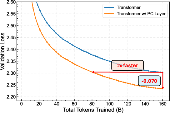
- With the AdamW optimizer: reaches the same loss using about half the training data (about 2× speedup).
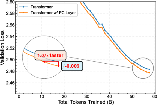
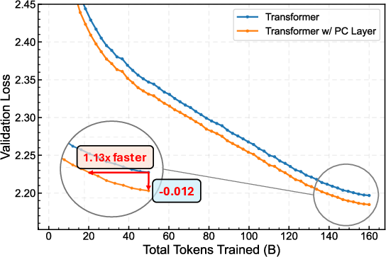
- With the Muon optimizer: about 1.13× speedup.
- Better accuracy on standard tests
- The 1B model with PC scored higher on average across common zero-shot benchmarks (like LAMBADA, HellaSwag, and ARC) for both AdamW and Muon.
- Healthier weight “shape”
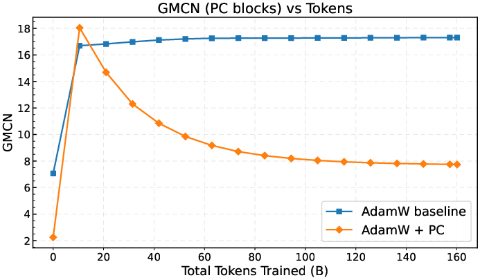
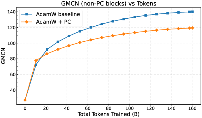
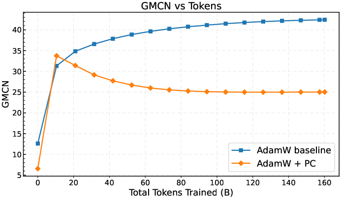
- They measured a stable version of the condition number (a way to quantify how unbalanced the weights are). With PC, this number went down a lot, showing the weights became better balanced and more stable for signal flow.
- Low overhead during training, zero overhead when using the model
- Extra compute during training was tiny (well under 1% FLOPs in their setup), a moderate increase in memory, and no extra cost when running the trained model.
Why this matters: Better-balanced weights help signals move smoothly through very deep models. That usually means easier optimization, less chance of training instabilities, and faster progress to good performance.
5. Why is this important?
- It makes big models easier and faster to train
- If you can reach the same quality with fewer training tokens, you save time and money.
- It’s simple and plug-and-play
- It changes how weights are used during training, not the overall architecture, and adds no cost at inference.
- It balances flexibility and stability
- Unlike methods that try to force every weight to act the same (which can hurt what the model can represent), the PC layer gently narrows the gap without flattening everything. This keeps the model expressive while making training smoother.
- It comes with theory
- The authors prove (in a simplified setting) that when each layer’s weights are well-balanced, plain gradient descent can reach the global best solution quickly. This supports the idea that “good weight spectra” help optimization.
Key terms in plain language
- Weight matrix: A big table of numbers in a neural network layer that decides how inputs turn into outputs.
- Singular values: Imagine the layer pushes information along many directions; each direction has a “loudness” number. These loudness numbers are the singular values.
- Condition number: The ratio of the loudest direction to the quietest direction. If it’s huge, signals get unevenly amplified or squashed, making training harder.
- Polynomial: A simple math function made of terms like a·x, b·x³, c·x⁵, etc. Here it’s used like a gentle, learnable equalizer to reshape loudness across directions.
In short, the PC layer is a small training-time tool that “equalizes” how layers pass signals. It helps big LLMs learn faster and more steadily, improves their test performance, and doesn’t slow them down when you deploy them.
Knowledge Gaps
Below is a concise, actionable list of knowledge gaps, limitations, and open questions left unresolved by the paper.
- Theory: The convergence guarantee is proved only for deep linear networks under (full-batch) gradient descent with bounded per-layer condition numbers; it does not cover nonlinear Transformers, attention, residual connections, stochastic training, or adaptive optimizers like AdamW/Muon. What conditions would extend the guarantee to realistic LLMs and optimizers?
- Theory–method link: There is no formal proof that the proposed polynomial PC layer actually maintains bounded condition numbers during training (with estimation noise, gamma scaling, optimizer dynamics). Can one derive sufficient conditions on the polynomial, normalization, and learning dynamics that ensure a persistent lower bound on σ_min and an upper bound on σ_max?
- Optimal spectrum shaping: The paper motivates avoiding exact orthogonality and proposes fixed piecewise-linear targets, but does not characterize optimal spectrum shapes per layer/depth/task. Can one derive task- or depth-dependent targets (or regularizers) that trade off expressivity and conditioning with theoretical or empirical optimality?
- Static vs adaptive PC: The polynomial, cutoff b, and pc_level are fixed globally. Would adaptive selection per layer and over training (e.g., schedule pc_level, data-driven fitting to current spectra, or per-layer targets) yield larger gains or avoid over-/under-shaping?
- Left vs right vs two-sided preconditioning: Only one-sided preconditioning is used (choose left or right by matrix shape). What are the effects of right-only and two-sided forms p(WWT)W, W p(WTW), or p_L(WWT) W p_R(WTW) on stability, compute, and quality?
- Polynomial design choices: The fitting uses a weighted least squares with weight w(σ)=σα, but α and sensitivity to this choice are not reported. How do different weighting schemes (e.g., minimax Chebyshev, alternative weights) and polynomial degrees trade accuracy, stability, and compute?
- Rational or other function classes: Only polynomials are explored. Could rational approximations, truncated Neumann series, or splines provide better conditioning with lower degree (compute) or improved robustness near σ≈0 and σ≈1?
- Spectral-norm estimation error: The streaming power-iteration estimator (10 iterations/step) is assumed accurate enough; there are no formal error bounds or analysis of how estimation noise propagates through gradients and stability. Can we bound estimator-induced drift and its impact on training, or amortize/refresh s(W) less frequently without loss?
- Sensitivity to the normalization margin: The polynomial is fitted on [0, 1.1] to accommodate s(W) error. What are the failure modes if σ exceeds this band (underestimation) or sits well below it (overestimation)? How tight must the margin be at scale?
- Role and dynamics of the learnable γ: The learnable per-block scalar γ stabilizes magnitude but its dynamics (e.g., learned distribution, coupling with optimizer, sensitivity to initialization) are not analyzed. Would alternative scalings (per-head, per-row/column, or vector scaling) be more effective or stable?
- Where to apply PC: PC is applied to FFN and W_O only. What is the effect of applying PC to W_Q/W_K/W_V, embeddings, output heads, or all linear maps? Can selective application (e.g., only deeper layers) improve compute–gain trade-offs?
- Interaction with existing normalizations: The compatibility and combined effects with RMSNorm, QK-Norm, weight decay, gradient clipping, and other weight-space constraints (row/column norms, hypersphere/hyperball, spectral sphere) are not systematically studied. Are there synergies or conflicts (e.g., duplicated control of logit or feature scales)?
- Comparisons to alternative weight controls: No head-to-head comparisons with strong baselines like spectral normalization, orthogonal/Householder parameterizations, Cayley transforms, sign/polar maps, or recent spectral/row–column constraints in LLMs. Which regimes favor PC over these alternatives?
- Scale and generality: Results are limited to Llama-271M and 1B on FineWeb. Do benefits persist or improve at 7B–70B scale, different token budgets, multilingual/code corpora, vision/multimodal Transformers, or MoE architectures?
- Robustness and variance: There is no report of variability across random seeds, confidence intervals, or statistical significance for validation loss and downstream accuracy. How stable are the gains across seeds and hyperparameter perturbations?
- Wall-clock vs token-efficiency: The paper reports token-efficiency but not end-to-end wall-clock speedups. Given memory overhead and added matmuls, do we see net time-to-target improvements on real training stacks and diverse hardware (H100, A100, TPU)?
- Memory overhead at scale: Peak memory overhead is ~9–10% at 1B. How does this scale with model size, sequence length, tensor/pipeline parallelism, activation checkpointing, and optimizer states? Can memory be reduced (e.g., recomputation, lower-degree polynomials, sparse evaluation)?
- Distributed training integration: The impact of PC on tensor/pipeline/sequence parallelism and ZeRO sharding is not addressed. How should g(W) be computed when W is sharded across ranks, and what are the communication costs?
- Frequency of s(W) updates: s(W) is estimated every step with 10 PI iterations. Could we safely reuse s(W) across multiple steps, maintain EMA/momentum estimates, or adapt PI iterations dynamically to reduce overhead without degrading results?
- Numerical precision: The effect of BF16/FP8 mixed precision on polynomial evaluation stability and spectral shaping is not reported. Are there precision-specific instabilities or mitigation strategies (e.g., Kahan summation, rescaling) for high-degree polynomials?
- Compatibility with post-training workflows: The impact on quantization (8/4-bit), pruning/sparsification, KV cache compression, and PEFT/LoRA fine-tuning is unknown. Does storing PC(W) alter quantization error, sparsity patterns, or adapter effectiveness?
- Downstream breadth: Zero-shot evaluation covers nine tasks; no few-shot, chain-of-thought, long-context, multilingual, or safety/reasoning benchmarks are reported. Do PC-induced spectrum changes transfer to broader downstream capabilities?
- Over-flattening boundary: While an appendix stress test suggests over-flattening can hurt, there is no principled criterion to detect or prevent “too-strong” shaping during training. Can we monitor a proxy (e.g., layerwise GMCN thresholds) and automatically attenuate pc_level?
- Global metric validity: The modified condition number uses the average of the bottom 10% singular values. Is this choice robust across shapes and layers? How sensitive are conclusions to this percentile and do alternative robust metrics correlate better with loss improvements?
- Causality vs correlation: The paper shows reduced GMCN co-occurs with improved optimization, but does not isolate causal links. Can interventions (e.g., forced spectrum shaping without other changes) establish causality and identify minimal necessary spectrum changes?
- Applicability to non-Transformer blocks: It remains unclear whether PC benefits convolutional layers, recurrent layers, or adapters. Are there architecture-specific polynomials or targets better suited to these modules?
- Safety/robustness under distribution shift: No experiments assess robustness to domain shift, adversarial/noisy data, or curriculum changes. Does spectrum shaping improve or hurt robustness and calibration?
- Hyperparameter selection: pc_level is chosen differently for AdamW and Muon via ablations; there is no principled selection rule. Can we predict pc_level from observed spectra or use a controller to set it online per layer?
These gaps highlight concrete avenues for future work, including theoretical extensions to realistic training settings, adaptive and per-layer PC policies, broader empirical validation and comparisons, improved efficiency/precision strategies, and careful integration with large-scale distributed training and downstream workflows.
Practical Applications
Immediate Applications
The following applications can be deployed now using the paper’s code and methods, with minor engineering effort.
- LLM pre-training acceleration and stabilization (software/AI, cloud, industry R&D)
- What: Integrate the PC layer into Transformer pre-training to reshape weight spectra during training, reducing token requirements and improving stability without inference-time overhead.
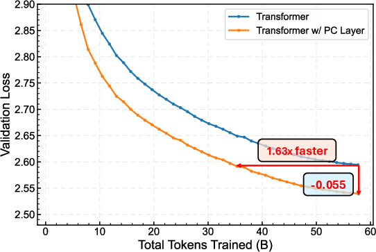
- Why it matters: Demonstrated token-efficiency speedups on Llama-1B (≈2× with AdamW; ≈1.13× with Muon), lower final loss, and improved zero-shot accuracy on 8/9 tasks.
- How: Add the PC layer to FFN and attention output projection (W_O) matrices; select
pc_levelper optimizer (e.g., 4 for AdamW, 2 for Muon); use streaming power iteration (≈10 steps) for spectral norm estimation; fold preconditioned weights into the model at the end of training. - Tools/workflows: PyTorch integration (TorchTitan-compatible), Horner’s method for evaluating polynomials; export weights normally (no inference overhead).
- Assumptions/dependencies: Results validated at 271M and 1B scales on FineWeb; generalization to larger models (e.g., 7B–70B) or other datasets likely but unproven; 0.24–0.39% FLOPs overhead and ≈9% peak training memory overhead; streaming spectral-norm estimation accuracy must remain within the design interval.
- Cost and energy/carbon reduction for foundation-model training (cloud, energy/sustainability, enterprise)
- What: Achieve same validation loss with fewer tokens/GPU-hours, lowering compute cost and emissions.
- Tools/workflows: Integrate PC into existing training pipelines; track token efficiency and energy usage per run.
- Assumptions/dependencies: Cost/emissions benefits depend on actual hardware mix and energy sources; modest training memory overhead may affect batch-size choices.
- Robust spectrum-health monitoring in training (ML Ops/tooling)
- What: Use the paper’s Modified Condition Number (per-layer) and Global Modified Condition Number (GMCN) as training-time health metrics to detect and mitigate spectral pathologies (e.g., collapsing tails, instability).
- Tools/workflows: Add periodic singular-value sampling or approximations (e.g., power iteration) to dashboards; trigger alerts or automatically adjust
pc_levelif GMCN degrades. - Assumptions/dependencies: Extra monitoring incurs minor compute; use bottom-10% averaging to avoid numerical fragility.
- Training on constrained budgets and smaller labs (academia, startups)
- What: Use PC to improve token-efficiency and stability when resources are limited, enabling more experiments per budget.
- Tools/workflows: Drop-in PC layer with baseline-tuned LR (paper keeps LR from the baseline), minimizing tuning overhead.
- Assumptions/dependencies: Memory overhead may require reducing per-GPU batch size; tested optimizers: AdamW and Muon.
- Apply to other Transformer modalities and finetuning (vision, speech, code; enterprise product teams)
- What: Extend PC to Transformer-based training outside LLMs (e.g., ViTs, speech encoders) and to finetuning large models for domains (healthcare, finance, education).
- Tools/workflows: Start with the same layer choices (FFN and W_O) and conservative
pc_level; monitor GMCN and downstream validation. - Assumptions/dependencies: Not explicitly evaluated in the paper; need pilot runs to confirm gains; datasets and layer shapes differ; streaming norm estimation must be calibrated.
- Safer mixed-precision/long-context training (ML systems)
- What: Use PC’s spectrum control to reduce gradient/activation extremes that can cause NaNs/instability under mixed precision or very long sequence lengths.
- Tools/workflows: Combine with FP16/bfloat16/FP8 and long-context schedules; monitor GMCN and loss spikes.
- Assumptions/dependencies: Evidence is indirect; stability improvements are plausible but need case-by-case verification.
- No-overhead deployment for AI products (software, edge, embedded)
- What: Because PC is a training-time reparameterization with weights folded post-training, inference-time latency and memory remain unchanged.
- Tools/workflows: Include a “fold-weights” step in model export; validate parity between training and exported weights.
- Assumptions/dependencies: Ensure the recovery scalar and learnable γ are folded correctly; add a regression check in CI.
Long-Term Applications
These applications require further validation, scaling studies, or development of tooling and theory.
- Standardized spectrum-aware training stacks (software/AI frameworks, hardware vendors)
- What: Make PC (or variants) a default module in PyTorch/DeepSpeed/Megatron training templates, with fused kernels for Gram-polynomial evaluation and streaming norm estimation.
- Potential products: “PC Layer” plugin with CUDA kernels; optimizer wrappers that co-tune
pc_level. - Dependencies: Kernel engineering for large-scale efficiency; benchmarking on 7B–70B+ models, MoE architectures, and diverse datasets.
- AutoPC: Adaptive per-layer polynomial and schedule (AutoML)
- What: Automatically fit or select preconditioning polynomials per layer and training phase, guided by GMCN trajectories and validation metrics.
- Potential products: Controllers that modulate
pc_level, target cutoffs, or layer coverage over time. - Dependencies: Fast on-the-fly spectral statistics (sketching/low-rank approximations); safeguards against over-flattening.
- Quantization- and compression-aware training (edge/serving, model compression)
- What: Use PC to produce better-conditioned weights that may quantize/compress more robustly (INT8/FP8/PTQ/QAT) and reduce accuracy loss.
- Potential workflows: Apply PC late in training; evaluate post-training quantization error and calibration stability.
- Dependencies: Empirical studies across quantization schemes; may need polynomial targets tailored for quantization resilience.
- Theory-informed convergence and generalization (academia)
- What: Extend the paper’s deep-linear convergence guarantees to nonlinear Transformers; study links between spectrum control, generalization, and representation anisotropy.
- Potential tools: Analytical bounds; new target maps beyond piecewise-linear; layer-wise theory-guided policies.
- Dependencies: Nonlinear theory remains open; empirical-theory feedback loop needed.
- Training stability for RL and robotics foundation models (RLHF/RLAIF, policy learning, robotics)
- What: Apply spectrum control in unstable regimes (off-policy RL, long-horizon credit assignment) to reduce gradient pathologies.
- Potential workflows: Combine with PPO/IMPALA variants; monitor GMCN during policy/value network training.
- Dependencies: Limited evidence to date; additional RL-specific evaluation and kernel adaptations.
- Spectrum-health governance and compute policy (policy, compliance, sustainability)
- What: Incorporate token-efficiency and GMCN-based health metrics into compute-governance frameworks to encourage energy-efficient, stable training practices.
- Potential tools: Reporting standards, audits, and SLAs that include spectrum-health indicators; procurement guidelines favoring spectrum-aware pipelines.
- Dependencies: Community and regulator consensus; reproducible metrics across frameworks.
- Robustness and safety research (security/reliability)
- What: Investigate whether better-conditioned weights reduce adversarial fragility, training instabilities, or catastrophic forgetting in continual learning.
- Potential workflows: Evaluate adversarial/perturbation robustness pre- and post-PC; integrate with LoRA/adapter finetuning.
- Dependencies: No direct evidence yet; requires systematic studies across tasks and threat models.
- Mixed-precision and low-precision training co-design (hardware/ML systems)
- What: Co-design PC with FP8 or block floating-point schemes to keep numerical ranges well-conditioned, reducing overflows/underflows.
- Potential products: Precision schedulers informed by GMCN; joint loss-scaling and spectrum-control strategies.
- Dependencies: Hardware support and kernel implementations; validation at scale.
- Curriculum and workforce training (education)
- What: Use PC and its spectrum-control perspective to teach practical numerical linear algebra for deep learning, linking theory to measurable training gains.
- Potential tools: Teaching labs, visualization of GMCN over training, polynomial fitting exercises.
- Dependencies: Educational material development and adoption.
Cross-cutting assumptions and dependencies
- Empirical scope: Demonstrated on Llama-271M and 1B with FineWeb; behavior at much larger scales, other modalities (vision/speech), and specialized architectures (MoE, retrieval-augmented) needs validation.
- Optimizer interactions: Tested with AdamW and Muon; other optimizers may require different
pc_levelor layer coverage. - Estimation accuracy: Streaming power iteration must keep spectral-norm estimates within the polynomial’s design interval; otherwise, out-of-domain evaluations can degrade results.
- Overheads: Training-time memory increases (~9–10% peak per GPU) may affect batch size; FLOPs overhead is small (~0.24–0.39%) but non-zero.
- Theory gap: Formal convergence guarantees currently hold for deep linear networks; nonlinear Transformer guarantees are an open research area.
Glossary
- AdamW: An optimizer that decouples weight decay from the gradient-based update in Adam, often improving generalization. "for both the AdamW and Muon optimizers."
- adjoint transformation: The transpose (or conjugate transpose) of a linear operator; in backpropagation, gradients propagate via the adjoint. "The same singular values also govern the adjoint transformation that appears in backpropagation."
- auto-differentiation: A technique to compute exact derivatives of programs efficiently by applying the chain rule through the computation graph. "are embedded into the network so that auto-differentiation applies to normalization layers."
- batch normalization: A layer that normalizes activations within a mini-batch to stabilize and accelerate training. "Representative examples include batch normalization"
- Chinchilla compute-optimal guideline: A heuristic relating tokens and model parameters for compute-optimal training in LLMs. "well above the Chinchilla compute-optimal guideline (20 tokens/parameter)"
- condition number: Ratio of largest to smallest singular value of a matrix; measures sensitivity and numerical conditioning. "if all weights of a multi-layer fully connected network have upper bounded condition number, then gradient descent converges to global minimizer at a rate dependent on the weight condition numbers."
- conjugate gradient: An iterative algorithm for solving large symmetric positive-definite linear systems using conjugate directions. "speeding up iterative methods such as conjugate gradient."
- cosine learning-rate schedule: A learning-rate schedule that decays the LR following a cosine curve, typically with warmup. "We use a cosine learning-rate schedule with linear warmup"
- dynamical isometry: A property where layers are near-isometric, preserving norms and enabling stable signal propagation through depth. "This connects weight-spectrum control to the classical dynamical-isometry and orthogonal-initialization literature"
- feed-forward network (FFN): The MLP sub-block in Transformers, typically comprising gate, up, and down projection matrices. "In the Llama~2 architecture, , , and refer to the three linear projections in the feed-forward network (FFN): the gate (gate_proj), up (up_proj), and down (down_proj) matrices, respectively."
- geometric convergence: Convergence at a linear (exponential) rate per iteration, reducing error by a fixed factor each step. "ensures geometric convergence of gradient descent to global minima"
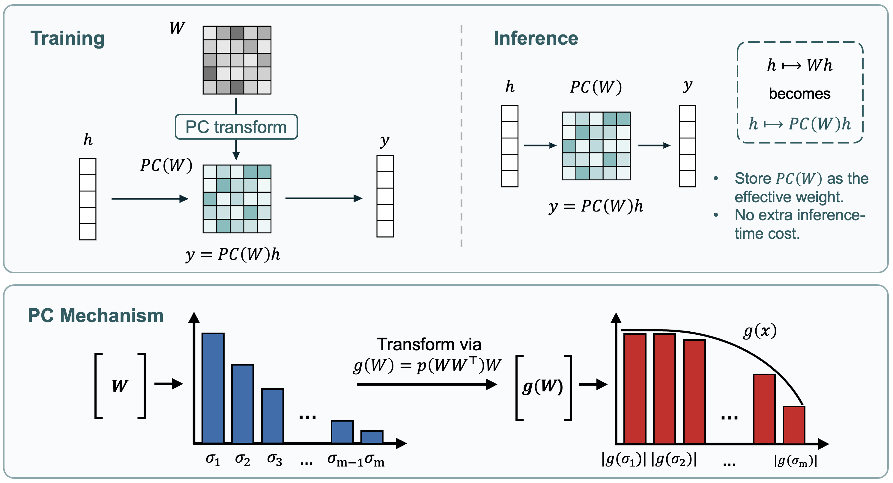
- Gram matrix: A symmetric matrix like or whose eigenvalues are the squared singular values of . "Polynomials are not directly defined on a rectangular , so we work through a symmetric Gram matrix"
- Horner’s method: An efficient scheme for evaluating polynomials using nested multiplications, reducing FLOPs. "The polynomial preconditioner can be computed efficiently via Hornerâs method"
- hyperball/hypersphere constraints: Constraints that force weight vectors to lie on or within a sphere to control their norms. "hyperball/hypersphere constraints on weights"
- Modified Condition Number: A robust conditioning metric using the top singular value over the average of the smallest 10% of singular values. "we introduce a Modified Condition Number metric, denoted as "
- muP-style spectral analyses: Analyses based on μ-parameterization that study spectral scales under width scaling. "This viewpoint is also compatible with P-style spectral analyses"
- Muon (optimizer): An optimizer designed for stable LLM training that often encourages near-orthogonal updates. "We further evaluate PC under Muon, a second widely used optimizer for LLM pre-training."
- orthogonal initialization: Initializing weights as (near-)orthogonal matrices to preserve signal norms at initialization. "The line of work on orthogonal initialization further refines this principle by providing a more fine-grained analysis of how depth affects signal propagation"
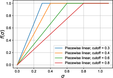
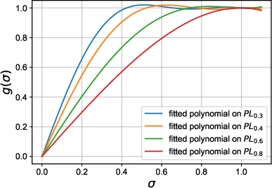
- piecewise-linear target: A simple function with linear segments used as a desired mapping to shape singular values. "This motivates the piecewise-linear target"
- polynomial preconditioning: Transforming a matrix by a polynomial in itself (or its Gram matrix) to alter its spectrum and improve conditioning. "Polynomial preconditioning is a classical technique in numerical linear algebra"
- preconditioning (PC) layer: A training-time weight-space module that reshapes singular values via a polynomial map to stabilize optimization. "We propose a preconditioning (PC) layer â a weight parameterization via polynomial preconditioner that ensures stable weight conditioning throughout LLM training."
- Query–Key Normalization (QK-Norm): A normalization applied to attention queries and keys to control logits and stabilize training. "QueryâKey Normalization (QK-Norm) \citep{henry2020query, loshchilov2024ngpt} has been widely used to control attention logits and stabilize training."
- RMSNorm: A normalization technique that rescales activations by their root-mean-square, commonly used in LLMs. "RMSNorm \citep{zhang2019root}, a variant of LayerNorm \citep{ba2016layer}, has become a de facto standard in most prevalent LLM architectures"
- sign/polar-style maps: Matrix transforms based on sign or polar decomposition that push singular values toward one (near-orthogonalization). "Unlike sign/polar-style maps (e.g., those used in Muon) that drive nearly all nonzero singular values toward one, PC performs soft spectrum shaping rather than near-orthogonalization."
- singular value decomposition (SVD): A factorization W = U diag(σ) Vᵀ expressing a matrix via singular vectors and singular values. "a singular value decomposition (SVD) "
- singular-value spectrum: The set or distribution of a matrix’s singular values, governing amplification/attenuation of signals. "reshapes the singular-value spectrum of weight matrices via low-degree polynomial preconditioning."
- spectral constraints: Constraints that directly control spectral properties (e.g., singular values) of weight matrices. "spectral constraints on weights \citep{newhouse2025training, xie2026controlled}, etc."
- spectral normalization (SN): A technique that scales weights by (an estimate of) their spectral norm to control Lipschitz properties. "spectral normalization (SN) \citep{miyato2018spectral}"
- spectral norm: The largest singular value of a matrix; equals its operator 2-norm. "we rescale the preconditioned matrix by the spectral-norm estimate"
- streaming power iteration: An iterative method, run online during training, to estimate the top singular value (spectral norm). "computed via streaming power iteration"
- token-efficiency speedup: Achieving the same validation loss with fewer training tokens, indicating more efficient learning. "token-efficiency speedups under both optimizersâi.e., it reaches the same loss with fewer training tokens (2 with AdamW and 1.13 with Muon)"
- weight normalization (WN): A reparameterization that decouples weight magnitude from direction by normalizing weight vectors. "weight normalization (WN) \citep{salimans2016weight}"
- weighted least squares: A regression method that minimizes squared errors with per-sample weights to better fit specific regions. "Weighted least-squares solutions in "
Collections
Sign up for free to add this paper to one or more collections.