Optimal Transport Flow Matching by Design
Abstract: Flow matching models learn to transport samples from a simple prior distribution to a complex data distribution. When prior-data pairs are coupled via optimal transport (OT), the learned trajectories are straight and non-crossing, enabling fast, even single-step, generation. However, computing the OT coupling in high dimensions is intractable, and existing methods attempt to solve the OT problem, at the cost of persistent bias or significant overhead. Rather than solving for the OT coupling, we reformulate the problem. Once the prior is treated as a design choice rather than a fixed input, the OT coupling between prior and data is no longer unique. Many priors admit an OT-optimal identity coupling to the data, leaving us free to choose one that is also tractable to sample. We identify low-frequency projection of natural images as such a choice. The identity coupling between data and its low-frequency representation is empirically OT-optimal, the prior is structured enough to be sampled by a lightweight model at inference, and the remaining flow-matching task reduces to synthesizing high-frequency detail. Interpolating the prior with Gaussian noise further improves generation quality while preserving the OT coupling. The approach requires no modifications to the flow model itself, and integrates naturally with latent-space models, classifier-free guidance, and one-step generation frameworks. Across all benchmarks, our method reduces trajectory curvature by more than $2\times$ compared to existing flow matching methods, yielding better generation quality in the few-step regime.


Paper Prompts
Sign up for free to create and run prompts on this paper using GPT-5.
Top Community Prompts
Explain it Like I'm 14
Overview
This paper is about making image generators faster and better, especially when they only get a few chances (steps) to produce a picture. The authors show a clever way to set up the “starting point” for the generator so that the path from “simple stuff” (like blurry shapes) to a finished image is as straight and easy as possible. This means the model can make good images in fewer steps.
Goals
The paper tries to answer three simple questions:
- Can we make the journey from “easy to sample” to “realistic image” straight and smooth, so we need fewer steps?
- Is there a way to get the benefits of optimal transport (the best way to move things) without having to solve a hard math problem?
- Can we design a better starting point for generation that a small, fast model can create, while the main model fills in the details?
How it works
Key ideas
- Think of generating images as moving from a simple starting point to the final picture. If all paths are straight and don’t cross, a model needs fewer steps to get there.
- In theory, the best way to guarantee straight, non-crossing paths is to match each starting point to the right final image using “optimal transport” (OT). But solving OT exactly for high-resolution images is too slow and expensive.
- The trick: don’t solve OT—design it. Pick a smarter starting distribution so that pairing each image with its own starting point is already OT-optimal “by design.”
What starting point did they design?
- They use each image’s low-frequency version as the start. Low-frequency means the blurry, coarse part of the image with big shapes and colors, without the tiny details.
- Why this helps:
- Most of an image’s energy (in the math sense) lives in low frequencies, so the blurry version is actually a good summary.
- Pairing each image with its own low-frequency version leads to straight, non-crossing paths (empirically OT-optimal).
- A small, fast model can learn to generate these low-frequency images easily.
A tiny bit of noise helps
- If the starting points were perfectly tied to each image (deterministic), training can get unstable and overfit.
- So they blend the low-frequency image with some Gaussian noise. This spreads out the starting points slightly without losing the “match.”
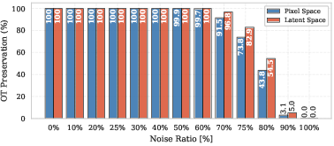
- They show that with a moderate noise level (about 50%), the “pair each image with its own low-frequency version” remains OT-optimal in practice.
Training and inference in simple steps
- Training:
- Make a low-frequency (blurry) version of each training image by downsampling and then upsampling.
- Mix this with some noise (a knob α controls how much).
- Train the main “flow matching” model to move from this starting point to the full, high-detail image along straight-ish paths.
Inference (making new images):
- A small, lightweight generator first creates a low-frequency image from random noise.
- Upsample it and add a bit of noise to form the starting point.
- The main model runs for just a few steps to add the fine details and produce the final image.
Explaining the technical terms
Flow matching: Teach a model a “velocity field” that tells it how to nudge an image step-by-step from a simple start to the final image.
- Optimal transport (OT): Imagine matching kids to seats so that the total walking distance is as small as possible. In images, it means pairing starting points and final images so the total “movement” is minimized, which makes paths straight and non-crossing.
- Low-frequency vs. high-frequency: Low-frequency is the broad shapes and smooth color regions (blurry version). High-frequency is the tiny edges, textures, and fine details (sharp version).
Main findings
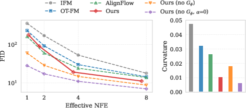
- Straighter paths: Across all tests, the method reduces “trajectory curvature” by more than 2× compared to standard flow matching approaches. Curvature is a measure of how bendy the path is; straighter paths mean fewer steps are needed.
- Better few-step quality: On CIFAR-10, FFHQ (faces), and ImageNet, the method improves image quality when you only allow a few steps. This is exactly where straight paths matter most.
- Works with popular tools: It plugs into common setups, including:
- Latent-space models (where images are generated in a compressed space).
- Classifier-free guidance (a standard trick to boost quality).
- One-step frameworks like MeanFlow, where it beats strong 1-step and 2-step baselines in their experiments.
- Noise sweet spot: A moderate noise mix (about α = 0.5) keeps the OT pairing intact and gives the best quality.
- Low-frequency is key: Other “projection” tricks that are OT-correct on paper but don’t preserve low-frequency structure don’t work as well. Keeping the coarse structure is crucial.
Why it matters
- Faster generation: Because the paths are straighter, you can get high-quality images with fewer steps—saving time and compute.
- Simple and practical: No need to run heavy OT solvers or change the model architecture. Just choose a better starting distribution.
- Flexible: It fits neatly into existing image generators and can boost single-step or few-step performance—useful for real-time apps or running on smaller devices.
- Broader impact: The idea of “OT by design” could inspire similar strategies for videos, audio, 3D, or any domain where you want fast, high-quality generation.
In short, the paper shows that by carefully choosing what the generator starts from (a blurry version of the target image plus a little noise), you can make the whole journey to a final, sharp image much simpler and straighter—leading to better results with fewer steps.
Knowledge Gaps
Knowledge gaps, limitations, and open questions
Below is a focused list of concrete gaps and open questions that remain unresolved and could guide future research.
- OT-optimality under practical projections: The paper provides empirical evidence (Hungarian matching) and a supplemental argument for strict orthogonal projections, but lacks a rigorous proof that bicubic downsampling (non-orthogonal, non-isometric) yields an identity OT coupling under squared Euclidean cost in high dimensions. When, and under what assumptions on the data distribution and operator T, is the identity coupling provably optimal?
- OT preservation with noise interpolation: The identity coupling is only empirically shown to persist up to α≈0.5 under finite-sample discrete OT. There is no theoretical characterization of how α, dimension d, and downsampling ratio jointly determine when the identity coupling remains optimal (or approximately optimal) for the noisy prior in Eq. (5). Can we derive guarantees or sharp thresholds for preservation as a function of d and the spectrum of p1?
- Coupling under alternative costs/metrics: The approach assumes squared Euclidean cost in pixel or latent space. It is unknown whether identity coupling remains optimal (or beneficial for curvature) under perceptual metrics, learned feature-space distances, or dataset-specific Riemannian metrics where Euclidean geometry is a poor proxy for semantic similarity.
- Distribution shift from prior mismatch: Training uses x0 = (1−α)T(x1)+αε with x1 from the dataset, but inference uses x0 derived from Gφ(z). The impact of mismatch between T#(p1) and the learned Gφ#(p0) on curvature and FID is not fully quantified. How robust is vθ to systematic errors in coarse structure from Gφ, and what failure modes occur when Gφ underfits or overfits?
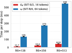
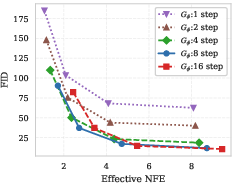
- Sensitivity to Gφ capacity and budget: The method introduces a second model Gφ and additional NFE. The paper reports small overhead, but does not map the trade-off between Gφ capacity/steps and final FID/curvature. What is the minimal Gφ complexity needed to sustain curvature and quality gains, and how does this scale with resolution and dataset complexity?
- Non-injectivity and multi-modality at α→0: T maps many x1 to similar or identical low-frequency representations; without sufficient noise, a single x0 may correspond to multiple x1 modes. Beyond empirical observations, there is no analysis of how much noise is needed to resolve multi-modality as data scale grows. Can we quantify mode-collision risk and its dependence on downsampling factor and dataset diversity?
- Path choice and training dynamics: The method retains linear interpolation paths. It is unknown whether alternative paths tailored to the projection (e.g., projection-aware or geodesic paths) could further reduce curvature or remove the need for α noise, especially near t≈0 where support lies on a low-dimensional subspace.
- Generality beyond natural images: The low-frequency prior leverages 1/f2 spectra of natural images. The approach is not evaluated on domains with different spectra or structure (e.g., line art, medical imaging, satellite SAR, text renderings). Does OT-by-design still hold, and which transform T is appropriate in such settings?
- Extensions to other modalities: Claims of broad applicability are not tested on audio, 3D, point clouds, or video. What are effective T operators for these modalities (e.g., temporal low-pass for audio/video, multiscale graph filters for meshes), and does identity coupling remain (approximately) optimal?
- Latent space implications: For FFHQ/ImageNet, operations are in VAE latents. It remains unclear how the choice of autoencoder (compression ratio, reconstruction loss, latent geometry) affects OT optimality and curvature. Are results sensitive to the latent metric and to latent-space “low-frequency” not aligning with pixel-space semantics?
- Conditioning and guidance integration: While compatibility with CFG and MeanFlow is claimed, there is no systematic study of conditioning-aware priors (e.g., class- or prompt-conditioned Gφ/T). Can conditioning be baked into the prior to further shorten flows, and how does guidance strength interact with curvature when starting from structured priors?
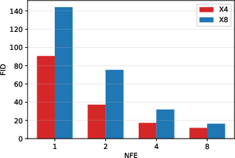
- Scaling to higher resolutions: Experiments stop at 256×256. It is unknown whether benefits persist (or grow) at 512–1024+ resolutions where low-frequency energy concentration is stronger but Gφ becomes harder to train. How should downsampling ratios and α scale with resolution?
- Choice and learning of T: Bicubic downsampling is selected over Fourier truncation for small empirical gains, but a principled method for choosing or learning T (e.g., learned orthogonal projections, steerable multiresolution transforms, content-adaptive filters) is missing. Can T be optimized to maximize OT identity preservation and sampleability while minimizing curvature?
- End-to-end training vs. staged training: The paper trains Gφ and vθ separately. It remains open whether joint or alternating training (with consistency or adversarial terms on the prior) reduces mismatch and improves few-step fidelity and stability.
- Noise calibration and schedules: Inference uses a “small noise perturbation” to x0 and a fixed α during training. The method lacks ablations or theory for time-dependent α schedules or adaptive perturbations near t≈0 that might improve stability on low-dimensional supports.
- Robustness, precision/recall, and diversity: Evaluation focuses on FID and curvature. Precision/recall or coverage metrics, out-of-distribution robustness, and diversity under strong structural priors are not reported. Does a strong low-frequency prior bias texture statistics or reduce fine-detail diversity?
- Computational and training cost: Although inference overhead is small, total training wall-clock and energy costs for two models (Gφ and vθ) are not compared against strong OT baselines (e.g., semi-discrete OT preprocessing). What is the end-to-end compute trade-off when accounting for both models, including hyperparameter sweeps for α and downsampling?
- Reliability of OT verification: The reported discrete OT verification uses the Hungarian algorithm on up to 10k samples, which is cubic in n and can be infeasible at larger n or higher d. How reproducible and scalable is this verification, and can approximate global checks (e.g., Sinkhorn with guarantees) validate OT identity preservation at scale?
- Interaction with one-step/few-step objectives: Integration with MeanFlow is promising but not systematic. How do consistency or shortcut objectives interact with OT-by-design priors, and can joint objectives be devised to explicitly penalize curvature while preserving the identity coupling?
- Theoretical links to Brenier maps: For continuous distributions, Brenier theory guarantees OT maps as gradients of convex functions. The conditions under which identity is the Brenier map to T#(p1) (beyond strict orthogonal projections) are not established. Can we characterize classes of linear and nonlinear T for which the identity is (approximately) the OT map?
Practical Applications
Immediate Applications
The following applications can be deployed with current image-generation pipelines using flow matching or one-step frameworks, with only minor engineering to add the prior-design module described in the paper.
- Sector: Creative media, advertising, gaming — Low-latency image generation in production
- What: Reduce GPU time and latency for text-to-image or image-to-image pipelines by replacing pure Gaussian priors with the paper’s low-frequency prior and few-step ODE solves. Demonstrated >2× trajectory straightening and better FID at few NFEs.
- Tools/workflows:
- Add a “PriorDesigner” module that performs
D(downsample/low-pass),U(upsample), and noise interpolation with α≈0.5 during training; train a lightweightG_φto sample low-res priors; keep the main flowv_θunchanged. - Integrate with classifier-free guidance (CFG) and single-step frameworks (e.g., MeanFlow) as shown in the paper.
- Assumptions/dependencies:
- Data are “natural image-like” with 1/f² spectral decay so low frequencies preserve most L2 energy.
- Autoencoder/latent quality (if using latent-space models) is high (e.g., Stable Diffusion VAE).
- α must be tuned; authors find α≈0.5 preserves the OT-identity coupling and minimizes FID.
- Sector: Consumer apps (mobile imaging, social, avatars) — On-device and edge generation
- What: Achieve acceptable-quality single/few-step image generation on mobile/edge by leveraging the coarse-to-fine prior and reduced curvature (better battery life, faster UX).
- Tools/workflows:
- Ship a small
G_φ(e.g., 1–8 steps) to generate an 8×8 or 16×16 latent prior on-device, then run 1–2 evaluations ofv_θ. - Optional: Tiny on-device CFG scaling; server-side refinement as a fallback.
- Assumptions/dependencies:
- Memory and compute constraints allow a small
G_φand a minimal number ofv_θevaluations. - Domain remains in-distribution for the pretrained flow model.
- Sector: Post-production and photo editing — Coarse-to-fine enhancement and upscaling
- What: Use the high-frequency synthesis stage (from low-frequency prior to full detail) for image enhancement or upscaling plugins where the model adds plausible detail from coarse inputs.
- Tools/workflows:
- Plugin that takes low-res/blurred images, upsamples to
U(x↓), adds calibrated noise, and runs 1–4 evaluations ofv_θto synthesize detail. - Assumptions/dependencies:
- Trained on the same domain (e.g., portraits vs. landscapes) to avoid hallucinated artifacts.
- Enhancement is generative (not guaranteed faithful restoration); require disclaimers in UX.
- Sector: MLOps/Model acceleration — Drop-in prior module for flows/consistency/MeanFlow
- What: A general-purpose SDK that wraps training loops to create OT-by-design priors and straightened trajectories, improving few-step quality without OT solvers.
- Tools/workflows:
- Training hooks to compute
T(x)=U(D(x)), buildx₀=(1–α)T(x)+αϵ, and trainG_φ+v_θ. - Inference wrapper reporting effective NFE and curvature metrics; knobs for α and
G_φbudget. - Assumptions/dependencies:
- Codebase supports minor data-loader transforms and a small auxiliary model
G_φ. - Monitoring includes FID and trajectory curvature to guard regressions.
- Sector: Sustainability and FinOps — Compute and energy savings
- What: Fewer ODE steps per image lower GPU hours and energy use; measurable reductions can be reported for sustainability KPIs and cost savings.
- Tools/workflows:
- Benchmark wall-clock and energy before/after; set internal targets for effective NFE.
- Assumptions/dependencies:
- Savings depend on workload mix (CFG strength, resolution, batch size) and
G_φcost (shown ≈9% of a main step per the paper).
- Sector: Academia (ML + vision) — Baselines for few-step flows and OT research
- What: Use OT-by-design as a clean baseline to study coupling, curvature, and few-step behavior without dataset-wide OT solvers.
- Tools/workflows:
- Course labs or benchmarks comparing IFM vs. OT-by-design vs. minibatch/global OT; curvature and FID plots with identical architectures.
- Assumptions/dependencies:
- Reproducibility requires access to the same datasets and standard architectures (e.g., SiT, CIFAR-10/FFHQ/ImageNet).
Long-Term Applications
These require further research, domain adaptation, or regulatory/validation work, but are natural extensions of the paper’s “design the prior” idea to other modalities and tasks.
- Sector: Video generation — Spatiotemporal priors for few-step video synthesis
- What: Extend the low-frequency prior to include low temporal frequencies (and spatial), producing OT-friendly couplings that shorten transport paths for video frames.
- Tools/products:
- Video
Dthat jointly low-passes time and space;G_φthat samples coarse spatiotemporal volumes;v_θrefines temporal details. - Assumptions/dependencies:
- Need empirical evidence that identity coupling remains near-optimal with temporal noise (α) and that low-frequency temporal structure dominates for target domains.
- Memory-efficient architectures for 3D (x,y,t) are required.
- Sector: 3D content, AR/VR, robotics simulators — Coarse-geometry priors
- What: Use low-resolution geometry (e.g., downsampled point clouds, coarse voxel grids) as priors and refine to high-frequency meshes/RSFs with a flow.
- Tools/products:
Das mesh/pointcloud decimator;Uas learned geometric upsampler;G_φsamples coarse shape;v_θadds fine geometry/textures.- Assumptions/dependencies:
- Must validate OT-identity coupling for geometric representations; may need domain-specific projections.
- Robustness to non-natural spectra (CAD-like, sharp edges) is uncertain.
- Sector: Audio/TTS/music — Spectral-prior acceleration
- What: Design priors from low-frequency (or low-mel) spectral bands, speeding few-step audio generation by focusing flows on high-frequency detail (transients, sibilance).
- Tools/products:
Das low-pass mel-spectrogram projection;G_φgenerates coarse spectrogram;v_θrefines to full-band audio; optional vocoder.- Assumptions/dependencies:
- Must empirically verify OT-identity preservation for audio; noise interpolation α may differ due to dimensionality and perceptual factors.
- Sector: Medical and scientific imaging — Guided high-frequency synthesis
- What: Use physically plausible, low-frequency priors (e.g., downsampled MRI/CT or deconvolved microscopy) and refine to high-resolution with controlled generative detail for speed or dose reduction.
- Tools/products:
- Clinical workflows where
Dcaptures safe coarse anatomy;v_θrestricted by priors/constraints to mitigate hallucinations. - Assumptions/dependencies:
- Strict validation for fidelity, bias, and safety; explainable uncertainty; regulatory approval.
- Domain spectra and priors may not follow natural-image assumptions; identity OT may not hold.
- Sector: Data-centric AI and privacy — Efficient synthetic dataset generation
- What: Generate large volumes of synthetic images with reduced compute, enabling faster iteration for privacy-preserving training and A/B experiments.
- Tools/products:
- Batch generators with OT-by-design priors; scheduling policies that exploit low effective NFE at scale.
- Assumptions/dependencies:
- Utility of synthetic data is task-dependent; requires bias/shift assessment and governance.
- Sector: Policy and standards — Energy-efficient generative AI benchmarks
- What: Introduce trajectory curvature and effective NFE as reporting metrics for procurement and sustainability standards; encourage “OT-by-design” practices to cut emissions.
- Tools/products:
- Benchmark suites publishing FID vs. effective NFE and curvature; checklists for prior design.
- Assumptions/dependencies:
- Needs consensus in standards bodies and reproducible public implementations.
- Sector: Secure and offline systems — Low-connectivity creative tools
- What: Offline-capable generative tools (e.g., field reporters, defense, remote communities) using few-step generation with small
G_φ. - Tools/products:
- Bundled models with compact
G_φ; adjustable α and step budgets for battery/runtime constraints. - Assumptions/dependencies:
- Model size and memory must meet device constraints; quality depends on domain fit.
- What: Offline-capable generative tools (e.g., field reporters, defense, remote communities) using few-step generation with small
- Sector: Foundation-model training — Curriculum via frequency-aware priors
- What: Pretrain flows with progressively richer priors (increase low-frequency bandwidth or decrease α) to stabilize and accelerate training.
- Tools/products:
- Training curricula that schedule downsampling factors and α; monitoring curvature reductions as a convergence signal.
- Assumptions/dependencies:
- Needs empirical studies across model scales and modalities to avoid overfitting to priors.
Cross-cutting assumptions and dependencies (affecting most applications)
- The OT-identity coupling is empirically validated (via Hungarian assignments) on natural-image datasets and holds up to moderate noise levels (α≈0.5). It is not theoretically guaranteed for all domains.
- Benefits rely on data having substantial low-frequency content; results may degrade for line art, schematics, or domains with dominant high-frequency structure.
- Quality depends on the lightweight prior generator
G_φ: too few steps or undercapacity can bottleneck the pipeline; however, the paper shows robustness even with 1–8G_φsteps. - Integrations in latent space inherit the quality of the autoencoder; compression artifacts can affect the effectiveness of the prior.
- Hyperparameters (downsampling factor, α, NFE split between
G_φandv_θ) require modest tuning per domain/resolution.
Glossary
- 1/f2 decay: A characteristic power-law falloff of energy with frequency observed in natural images. Example: "follows a decay~\cite{field1987relations,ruderman1994statistics}"
- Action minimization: A post-training procedure that straightens trajectories by minimizing a path cost functional. Example: "or action minimization~\cite{yue2025oat}"
- Anisotropic Gaussians: Gaussian priors with direction-dependent variance tailored to local data geometry. Example: "Anisotropic Gaussians capturing local manifold geometry~\cite{bamberger2025carr}"
- Autoencoder: A neural network that compresses data into a latent representation and reconstructs it back to the original space. Example: "operate in the latent space of a pretrained autoencoder~\cite{rombach2022stable_diffusion}"
- Blue noise: A noise distribution emphasizing high frequencies with minimal low-frequency content. Example: "time-varying blue noise~\cite{huang2024blue}"
- Cascaded diffusion: A multi-stage generative strategy that progressively increases resolution or detail across diffusion models. Example: "Cascaded diffusion~\cite{ho2022cascaded,saharia2022photorealistic}"
- Classifier-free guidance (CFG): A technique that steers generative models at inference without an explicit classifier by mixing conditional and unconditional predictions. Example: "classifier-free guidance (CFG)~\cite{ho2022classifier_free_guidance}"
- Cold Diffusion: A framework replacing stochastic noise corruption with deterministic degradations for generation. Example: "Cold Diffusion~\cite{bansal2023cold}"
- Consistency models: Models trained to produce consistent outputs across different integration steps, enabling few-step generation. Example: "Consistency models~\cite{pmlr-v202-song23a,yang2024consistency}"
- Entropic relaxations: Optimal transport solvers that add entropy regularization to the transport plan for computational tractability. Example: "entropic relaxations~\cite{NIPS2013_af21d0c9}"
- FID (Fréchet Inception Distance): A metric measuring the quality of generated samples by comparing feature distributions to real data. Example: "We report FID~\cite{fid} for generation quality"
- Flow matching: A training framework that learns a velocity field to continuously transport a base distribution to the data distribution. Example: "Flow matching~\cite{lipman2022flow,albergo2022building,liu2022flow}"
- Gaussian prior: A standard normal distribution used as the simple starting distribution for generation. Example: "between a high-dimensional data distribution and a standard Gaussian prior"
- Guided distillation: A distillation procedure that uses guidance signals to improve few-step or single-step generation. Example: "guided distillation~\cite{seongbalanced}"
- Hungarian algorithm: A combinatorial optimization method for computing exact assignments in discrete optimal transport. Example: "verify the resulting identity coupling is OT-optimal with the Hungarian algorithm"
- Identity coupling: A coupling that pairs each data point with its transformed counterpart via an identity map between spaces. Example: "The identity coupling between an image and its low-frequency representation is empirically OT-optimal"
- Latent diffusion: Generative modeling performed in a compressed latent space to reduce computational cost. Example: "latent diffusion~\cite{rombach2022stable_diffusion}"
- Latent space: A lower-dimensional representation space learned by an encoder where data structure is preserved. Example: "operate in the latent space of a pretrained autoencoder~\cite{rombach2022stable_diffusion}"
- Linear interpolation path: A simple path between source and target points given by convex combination over time. Example: "Under a linear interpolation path:"
- MeanFlow: A one-step or few-step generation framework optimizing mean-field approximations of the flow. Example: "MeanFlow~\cite{geng2025mean}"
- Minibatch OT: Approximating optimal transport by solving transport couplings within each training batch. Example: "Minibatch OT methods~\cite{pooladian2023multisample,tong2024improving}"
- Monge optimal transport problem: The formulation seeking a deterministic map that transports one distribution to another with minimal cost. Example: "The Monge optimal transport problem"
- NFE (Number of Function Evaluations): The count of model evaluations used to integrate or step through the generative process. Example: "Samples generated at $1$, $2$, and $4$ NFE."
- ODE (Ordinary Differential Equation): A continuous-time dynamical equation governing the evolution of samples along the learned flow. Example: "Ordinary Differential Equation (ODE)"
- Optimal transport (OT): A theory and set of methods for mapping one probability distribution to another with minimal cost. Example: "optimal transport (OT)"
- OT-identity coupling: The identity pairing between prior and data that is (empirically) optimal under the OT cost. Example: "empirically preserving the OT-identity coupling"
- Power spectrum: The distribution of signal energy across frequencies, often used to characterize images. Example: "The power spectrum of natural images follows a decay"
- Push-forward: The distribution induced by applying a map to a random variable. Example: "we denote the push-forward of by as "
- Pyramid flow: A generative approach that decomposes synthesis across multiple resolution scales in a flow framework. Example: "pyramid flow~\cite{jin2025pyramidal}"
- Score-based generative modeling: A paradigm learning the score (gradient of log-density) to sample data via stochastic differential equations. Example: "score-based generative modeling~\cite{song2019generative}"
- Semi-discrete OT: An optimal transport setting where one distribution is continuous and the other is discrete, enabling specialized solvers. Example: "semi-discrete OT approaches~\cite{kong2025alignflow,mousavi2025flow}"
- Spectral concentration: The phenomenon where most signal energy is concentrated in low frequencies. Example: "Leveraging the spectral concentration of natural images~\cite{ruderman1994statistics}"
- Trajectory curvature: A measure of how much learned transport paths deviate from straight lines; lower curvature implies straighter, faster trajectories. Example: "reduces trajectory curvature by more than "
- Velocity field: A time-dependent vector field specifying the instantaneous direction and speed of transport in flow matching. Example: "learns a velocity field that continuously deforms the simple distribution into the data distribution"
- Self-distillation: A process where a model is distilled from its own outputs to improve efficiency or trajectory straightness. Example: "through iterative self-distillation~\cite{liu2022flow}"
Collections
Sign up for free to add this paper to one or more collections.

