LLMs as Noisy Channels: A Shannon Perspective on Model Capacity and Scaling Laws
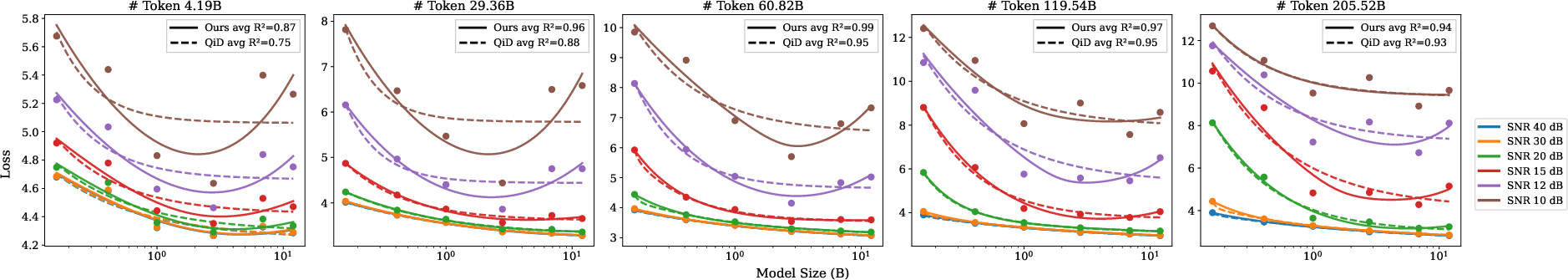
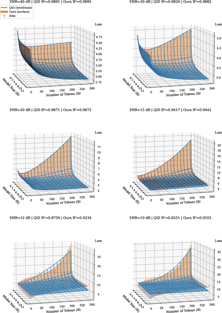
Abstract: Existing scaling laws for LLMs, predominantly monotonic power laws, fail to explain emerging non-monotonic phenomena such as catastrophic overtraining and quantization-induced degradation, where performance deteriorates despite increased compute. We propose the Shannon Scaling Law, a unified theoretical framework that models LLM training as information transmission over a noisy channel, grounded in the Shannon-Hartley theorem. By mapping model parameters to channel bandwidth and training tokens to signal power, our formulation explicitly captures the interaction between learning signal and intrinsic noise. This perspective reveals a fundamental Shannon capacity for LLMs: scaling model size or data without preserving a sufficient signal-to-noise ratio (SNR) inevitably amplifies noise, inducing a transition from monotonic improvement to U-shaped performance degradation. We validate our theory through experiments on Pythia and OLMo2 under perturbations, including Gaussian noise, quantization and supervised fine-tuning on math, QA and code tasks. The Shannon Scaling Law consistently outperforms classical scaling laws and recent perturbation-aware laws, achieving strong $R2$ scores and accurately capturing loss basins missed by prior approaches. It also extrapolates: fitted on $\leq$6.9B Pythia models with $\leq$180B tokens, it predicts the unseen 12B model up to 307B tokens at pooled $R2{=}0.847$, while monotonic baselines collapse.
Paper Prompts
Sign up for free to create and run prompts on this paper using GPT-5.
Top Community Prompts
Explain it Like I'm 14
What is this paper about?
This paper looks at how the performance of LLMs changes as we make them bigger and train them on more text. Instead of assuming “bigger is always better,” the authors use an idea from radio and Wi‑Fi (Shannon’s information theory) to explain why models sometimes get worse when we keep scaling them up. They propose a new “Shannon Scaling Law” that treats an LLM like a message sent over a noisy channel, where useful learning (signal) competes with various kinds of noise.
What questions are the authors asking?
The paper focuses on a few simple questions:
- Why do some models improve at first but then get worse when we keep training them or make them larger (a U‑shaped curve instead of a steady climb)?
- Can we build one simple rule (a scaling law) that explains both the usual case—where more size and data help—and the tricky cases—where more actually hurts?
- Can this new rule not only fit existing results but also predict how bigger, never-before-tested models will behave?
How did they study it? (Methods in everyday language)
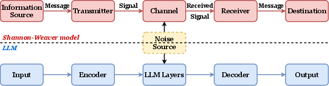
To make the ideas easy to picture, the authors compare LLM training to sending a song over a radio:
- Bandwidth: In radios, wider bandwidth lets you send more information. In LLMs, this is like model size—the number of parameters. Bigger models can store more.
- Signal power: In radios, stronger signal carries the song better. In LLMs, this is like the amount of training data (number of tokens). More tokens mean more chances to learn.
- Noise: Static that messes up the song. In LLMs, “noise” comes from:
- Messy data (typos, contradictions),
- The training process itself (models start noisy and get “cleaned up” over time),
- Limits you can’t avoid (architecture constraints, tiny errors).
Using the classic Shannon–Hartley formula from communication theory, they build a new scaling law (the “Shannon Scaling Law”) where:
- Capacity (how much useful knowledge the model can hold and use) grows with model size (bandwidth) and training tokens (signal),
- But it is reduced by different kinds of noise.
They then link capacity to test loss (how wrong a model is): roughly, higher capacity means lower loss.
To check if this law matches real life, they test on open-source model families (Pythia and OLMo2) across several situations:
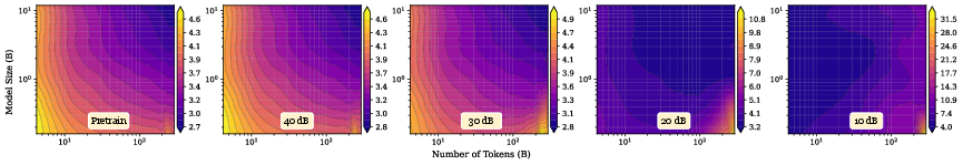
- Adding random “static” to model weights (Gaussian noise),
- Supervised fine-tuning (SFT) on math, QA, and coding tasks,
- Quantization (using fewer bits to store weights), which saves memory but adds errors.
They compare their law to well-known “monotonic” scaling laws (like OpenAI’s and Chinchilla’s) and newer “perturbation-aware” laws that try to account for noise.
What did they find, and why is it important?
Here are the key takeaways, explained simply:
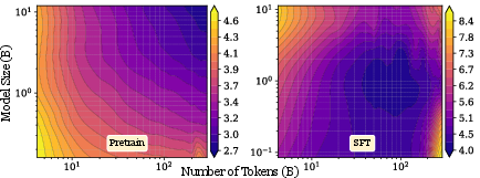
- U‑shaped behavior is real and predictable: In many noisy situations (heavy fine-tuning, low‑precision weights, added noise), performance first gets better with more size or data—but after a point it gets worse. This creates a “loss basin” (a sweet spot) rather than endless improvement.
- One law fits both worlds: The Shannon Scaling Law explains both:
- High‑quality pretraining with little noise (where “bigger and more data” usually helps),
- Noisy or stressed settings (where more can hurt).
- Better fits to data: Across many tests, their law fits the results more closely than older laws. It especially shines when things get noisy—where traditional laws often fail.
- It can predict the future (extrapolation): Trained only on smaller models and fewer tokens, their law successfully predicts how a larger, unseen model behaves with many more tokens. This is valuable for planning training runs without having to pay for all the experiments.
- A simpler version still works well: They also propose a smaller, easier-to-fit version of their law (fewer knobs to tune) that still performs strongly. Use this “simplified” version for single‑axis predictions (e.g., more tokens), and the full version for tougher, two‑axis predictions (bigger model and more tokens at once).
In short, the new law provides a more realistic view: performance depends on the balance between signal (useful data and capacity) and noise (everything that gets in the way). If noise grows faster than signal, scaling backfires.
What did the experiments show?
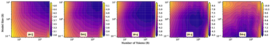
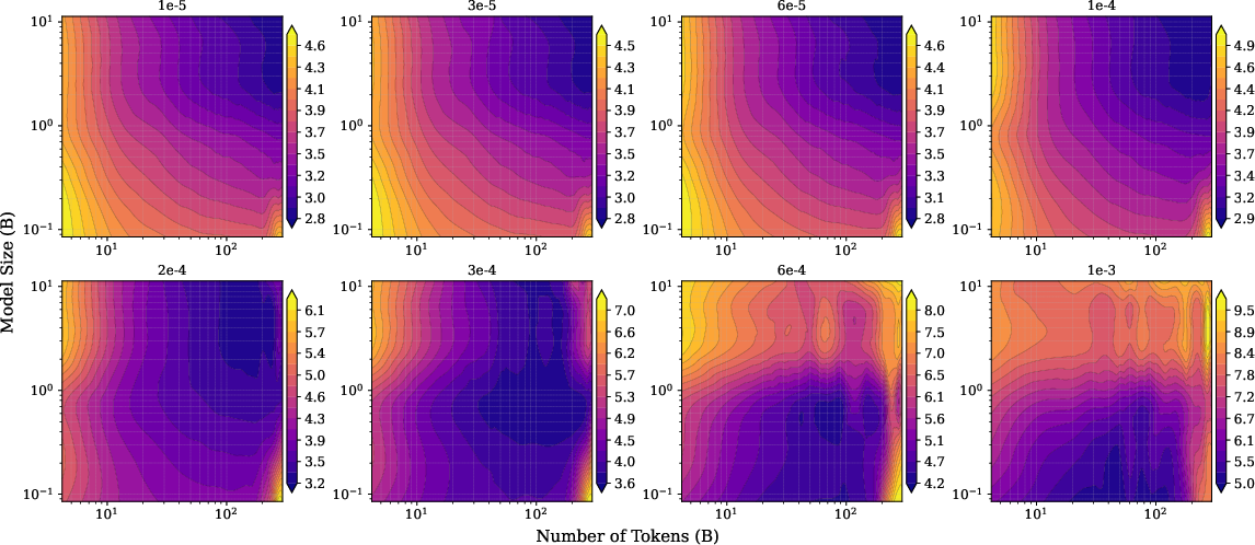
- With added random noise: Low noise → performance improves steadily; high noise → a U‑shape appears, and too many tokens or too large models start to hurt.
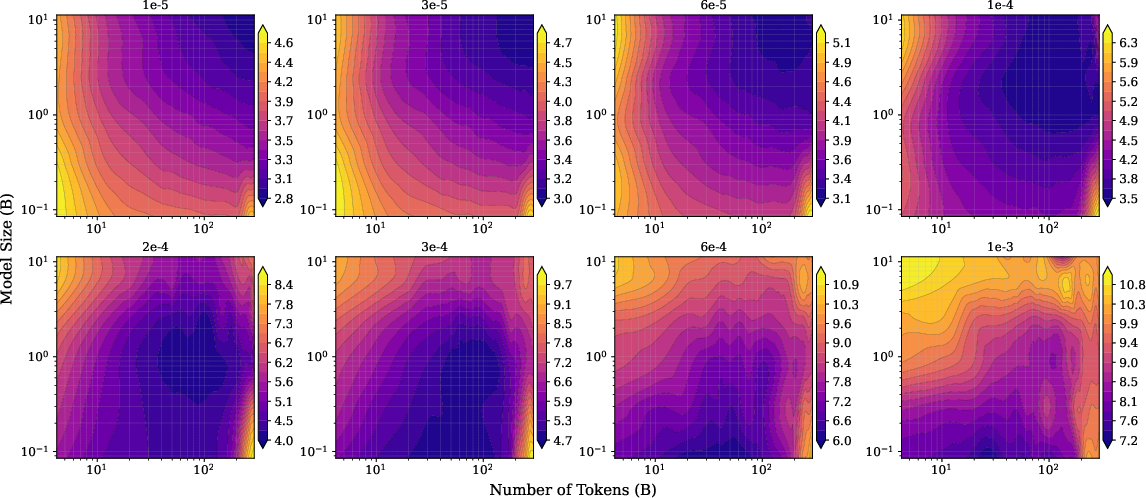
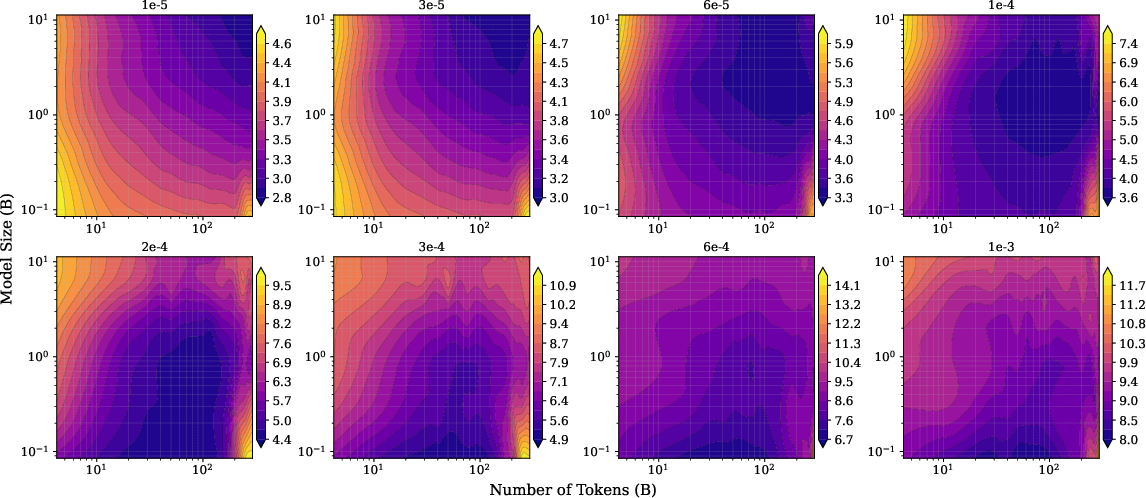
- With supervised fine-tuning: Small learning rates (gentle updates) behave well; large learning rates act like strong noise and cause “catastrophic overtraining,” where more training makes the model worse.
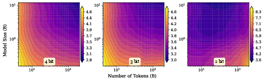
- With quantization: High precision (more bits) is okay; very low precision (2–3 bits) adds a lot of noise, and pushing size or tokens too far leads to worse results—again producing a U‑shape.
Why does this matter? (Implications)
This work helps researchers and engineers make smarter choices:
- Smarter scaling: Don’t assume “bigger and longer training” is always better. Watch the signal‑to‑noise balance and stop once you hit the sweet spot.
- Better training plans: Use the new law to plan model size, data amounts, learning rates, and precision so you don’t waste compute and money.
- Safer fine-tuning: Choose learning rates and training durations that avoid overtraining and the loss of earlier abilities.
- Practical quantization: Know when using fewer bits will break performance—and for which model sizes and data ranges it’s still safe.
- A unified theory: Instead of juggling separate rules for pretraining, fine‑tuning, and compression, this gives one framework that explains them all.
In everyday terms: Think of training an LLM like tuning a radio. Turn up the volume (more data) and buy a better radio (bigger model), but if the static gets too loud (noise from bad data, aggressive fine‑tuning, or low‑precision weights), cranking things up can actually make the music sound worse. This paper gives a practical formula for finding the right balance.
Knowledge Gaps
Knowledge gaps, limitations, and open questions
Below is a focused list of what remains missing, uncertain, or unexplored in the paper, phrased to guide concrete follow-up research.
- Theoretical grounding of the channel analogy:
- No formal derivation from learning theory showing that LLM loss should be proportional to the reciprocal of a Shannon–Hartley style capacity; the choice is heuristic and unvalidated against alternative link functions.
- The assumption of additive white Gaussian noise (AWGN) and the log(1+S/N) structure is imported from physical channels without proof that optimization dynamics and data/model noise in LLMs behave as AWGN or yield the same concavity and saturation properties.
- Lack of conditions under which the proposed capacity formula reduces to classical power-law scaling or produces U-shapes; no analytic characterization of the critical thresholds (in , , and noise) that trigger the monotonic-to-U-shaped transition.
- Identifiability and interpretability of parameters:
- The 9 fitted constants lack identifiability analysis; multiple parameter settings may fit equally well, risking over-parameterization.
- No uncertainty quantification (confidence intervals, posterior distributions, or sensitivity analyses) for fitted exponents and coefficients; unclear robustness of parameter values to data splits or noise in measurements.
- Exponent values are reported (partially) but not linked to interpretable architectural or data properties; unclear whether exponents transfer across perturbations or model families.
- Missing explicit perturbation variable in the unified law:
- The proposed Shannon Scaling Law does not include an explicit perturbation input (e.g., SNR in dB, quantization bit-width, or SFT learning rate); fits are performed separately per perturbation level, limiting the claim of “unification.”
- Open question: how to parameterize a single law with capturing perturbation magnitude/type, enabling one fit to predict across noise levels, LRs, and bit-widths.
- Validation beyond two model families and a narrow size range:
- Experiments are limited to Pythia (≤12B) and OLMo2 (≤32B stage-1 checkpoints); no evidence the law holds for larger frontier models, Mixture-of-Experts (MoE), or architectures with very different depth/width trade-offs or tokenizers.
- No tests on instruction-tuned, multilingual, or multi-modal models; generality across domains and modalities is unverified.
- Data and evaluation scope:
- Fits are primarily to wikitext2 test loss; relationship between the proposed capacity and downstream task performance (accuracy, reasoning metrics, code pass@k) remains unvalidated beyond using wikitext2 loss after SFT.
- Lack of multi-metric evaluation (e.g., calibration, long-context fidelity, factuality) to assess whether “capacity” correlates with broader quality attributes.
- Signal and noise modeling gaps:
- “Signal” assumed to scale as irrespective of data quality, duplication, domain mix, or curriculum; no measurement of effective information content versus token count.
- “Data-induced noise” and “model-interaction noise” are defined functionally (e.g., , ) but not empirically decomposed; no experiments estimating their separate contributions or validating their scalings.
- No operational estimate of SNR during real training; Gaussian weight noise injection calibrates SNR relative to weight power, but there is no mapping from training hyperparameters or quantization settings to an effective SNR.
- Noise realism:
- Injected noise is additive and weight-level; real perturbations (quantization, optimizer noise, activation/gradient noise, data corruption) are structured, layer-dependent, and often non-Gaussian.
- Quantization experiments are limited to PTQ (GPTQ) on weights; no evaluation of activation quantization, KV-cache quantization, group-size effects, per-layer sensitivity, or quantization-aware training (QAT).
- Training dynamics and compute constraints:
- The law abstracts training steps via but ignores optimizer, schedule, batch-size-induced gradient noise scale, regularization, and early stopping—all of which modulate effective noise.
- Compute-optimality is not revisited under the new law; there is no guidance for jointly choosing given a compute budget and noise regime to avoid entering the loss basin.
- Context and architectural factors not modeled:
- The “bandwidth” is mapped only to parameter count ; other capacity-critical variables (depth vs width, attention heads, hidden sizes, context window length, layer norms) are not incorporated.
- No analysis of how context length or sequence length during training/inference should enter the capacity term (e.g., as part of “bandwidth” or “signal”).
- Generalization and transferability of fits:
- Parameters are fit per model family and perturbation regime; there is no demonstration of parameter transfer across architectures, datasets, or perturbations (e.g., train on Pythia, predict OLMo2).
- Extrapolation is confined to within-family predictions up to modest scale; external validation on unseen architectures/datasets is missing.
- Statistical rigor:
- Model comparison relies on without penalizing for model complexity (e.g., AIC/BIC) or providing error bars; improvements could be due to higher parameter count rather than true explanatory power.
- No cross-validation across model sizes/tokens beyond the presented splits; limited analysis of overfitting risks on small grids.
- Practical thresholds and design rules:
- No closed-form or algorithmic procedure to locate the “safe region” and the loss-basin boundary for a given noise level; practitioners lack actionable criteria for choosing to stay at high SNR.
- Absent are interpretive diagnostics (e.g., per-layer SNRs or noise budgets) to guide interventions like data cleaning, layer-wise quantization, or schedule adjustments.
- Data quality and curation effects:
- The law does not model how deduplication, filtering, or domain balancing changes “signal” vs “data-induced noise”; no experiments varying data quality at fixed .
- Open question: can dataset entropy or mutual information estimates be used to refine the signal term?
- Mutual information link is not instantiated:
- Although the paper motivates capacity via , it does not measure mutual information or show that the proposed capacity correlates with MI estimates in practice.
- Edge cases and failure modes:
- Behavior for very small or extreme is not analyzed; conditions under which the law may fail (e.g., under-parameterized regimes, extreme curriculum shifts) remain unclear.
- Sensitivity to evaluation dataset choice is untested (e.g., domain mismatch between training data and wikitext2).
- Reproducibility and transparency:
- Key implementation details (e.g., per-layer noise injection specifics, quantization settings like group size/clipping, calibration data) are relegated to the appendix and only briefly referenced; code and fitted parameter releases are not indicated.
- Alternative functional forms:
- No comparison against other plausible concave link functions or information-theoretic capacity surrogates; it remains unknown whether simpler or differently structured non-monotonic forms could match or surpass performance with fewer parameters.
- Mapping perturbations to SNR:
- There is no calibrated mapping from quantization bit-widths, SFT learning rates, or other training perturbations to an effective SNR scale that would allow a unified, physically interpretable conversion.
- From fit to control:
- The framework is not used to design interventions (e.g., adaptive scaling of vs , dynamic LR schedules, noise-regularized training) that proactively avoid U-shaped degradation; no prospective validation of such control policies.
Practical Applications
Immediate Applications
These applications can be deployed now by leveraging the paper’s Shannon Scaling Law, its fitted exponents, and the demonstrated extrapolation behavior across model size, tokens, and perturbations (quantization, SFT, Gaussian noise).
- SNR-aware training budget optimization
- What: Choose model size (N), token budget (D), precision, and learning rate to stay in a high-SNR regime and avoid the U-shaped degradation region.
- Sectors: Software/AI labs, cloud ML platforms, finance (cost/performance planning), energy (compute efficiency).
- Tools/workflows: “Capacity planners” that fit the Shannon law on a small N×D grid; budget calculators that recommend N/D splits; dashboards showing predicted loss basins.
- Assumptions/dependencies: Requires a small grid of runs to fit parameters; extrapolation is strongest when both N and D axes are covered. Validated primarily on Pythia/OLMo2 and wikitext2 loss.
- Fine-tuning guardrails (learning rate and token scheduling)
- What: Use the law to set LR ranges and token budgets for SFT, with early-stop triggers when predicted capacity declines (catastrophic overtraining risk).
- Sectors: Enterprise software, education technology (domain-specific fine-tuning), healthcare and finance (safety-critical adaptation).
- Tools/workflows: LR schedulers that keep effective SNR above threshold; automatic “loss basin” detection; per-task fitted exponents to decide whether to scale N or D.
- Assumptions/dependencies: Mapping LR to noise is empirical; effectiveness may vary by task/optimizer; supervision signal and evaluation metric must align with the fitted loss.
- Quantization-aware model selection and deployment
- What: For edge/mobile or large-scale serving, select bit-width, model size, and training state that maximize capacity; prioritize less-overtrained/smaller models for low-bit deployments.
- Sectors: Robotics, mobile/edge AI, embedded healthcare devices, consumer software.
- Tools/workflows: Quantization policy recommender that predicts degradation across 2–4 bit; pipelines that adjust fine-tuning or lightweight retraining before quantization to stay in high-SNR zones.
- Assumptions/dependencies: Validated with GPTQ; other quantizers/activation quantization may shift the noise profile; downstream task alignment must be checked.
- Data curation prioritized by signal-to-noise
- What: Estimate the contribution of data-induced noise (Dδ term) to decide when additional tokens help vs. hurt; filter or reweight noisy subsets to strengthen SNR.
- Sectors: Data vendors, foundation model builders, public-sector data programs.
- Tools/workflows: Dataset SNR estimators tied to the law’s noise terms; automatic sampling and mixture policies to slow growth of data-induced noise.
- Assumptions/dependencies: Requires proxy metrics for noise in heterogeneous corpora; law is fitted on loss not direct “noise labels.”
- Extrapolative benchmarking to reduce compute
- What: Fit the simplified Shannon law (6 parameters) on small runs to predict larger-token or larger-model performance; use the full law (9 parameters) for joint N×D extrapolation.
- Sectors: Academia, startups, public research labs, cloud providers.
- Tools/workflows: “ShannonFit” library integrated with PyTorch/DeepSpeed that ingests small grids and outputs predicted performance; report pooled R² to prevent cherry-picking.
- Assumptions/dependencies: The full law requires coverage on both axes to outperform simpler forms; architectural shifts can break extrapolations.
- Checkpoint/model selection for downstream deployment
- What: Among training checkpoints, choose those with highest predicted capacity for target constraints (bit-width, LR/LoRA stacking); avoid late checkpoints if they enter the loss basin.
- Sectors: MLOps, platform engineering, SaaS providers.
- Tools/workflows: Capacity-aware checkpoint scoring; automated rollback when predicted capacity deteriorates.
- Assumptions/dependencies: Requires consistent evaluation metric across checkpoints; downstream tasks may respond differently than perplexity.
- Production monitoring and drift alarms
- What: Track effective SNR surrogates (e.g., increase in data-induced noise, new perturbations from adapters) and alert when capacity is predicted to drop.
- Sectors: Enterprise AI, regulated industries (healthcare, finance).
- Tools/workflows: Capacity-forecast dashboards; SNR-based service-level objectives (SLOs) tied to retraining or de-quantization actions.
- Assumptions/dependencies: Must map operational changes (plugins, adapters, guardrails) to noise terms consistently.
- Noise stress testing as a benchmarking standard
- What: Routine evaluations that inject Gaussian noise, vary precision, and sweep LR to chart loss basins and SNR regimes for model releases.
- Sectors: Model evaluation labs, model vendors, open-source communities.
- Tools/workflows: Automated perturbation harnesses; reports including fitted parameters and basin visualizations.
- Assumptions/dependencies: Gaussian/AWGN is a simplification; real-world perturbations may be structured (e.g., quantization plus activation clipping).
- Procurement and compute ROI calculators
- What: Forecast marginal returns of more compute or data using the law; prioritize runs with maximal capacity gains per dollar/watt-hour.
- Sectors: Finance (CapEx/OpEx planning), public-sector procurement, cloud resellers.
- Tools/workflows: Portfolio planners that compare N vs. D expansion; scenario analyses for precision trade-offs.
- Assumptions/dependencies: Needs historical fits and consistent cost models for hardware/energy.
- End-user guidance for local/edge LLM use
- What: Practical recommendations—prefer slightly smaller or less-overtrained models for aggressive 3–2 bit quantization; avoid cranking LR during SFT.
- Sectors: Daily life (developers/hobbyists), SMEs.
- Tools/workflows: Interactive wizards that propose a model–precision–finetuning plan with expected capacity drop.
- Assumptions/dependencies: Simplifies many factors (task mix, prompts, decoding); fit quality may degrade for very different domains.
Long-Term Applications
These directions require more research, scaling, standardization, or co-design beyond what is demonstrated in the paper.
- Closed-loop, capacity-aware training controllers
- What: Automated systems that continuously estimate capacity/SNR and adjust N, D, LR, precision, and training duration in real time; expand or shrink models dynamically.
- Sectors: Cloud training platforms, hyperscalers, foundation model vendors.
- Potential products: “Capacity autopilot” for training; compute orchestration that avoids loss basins.
- Dependencies: Online, low-variance capacity estimation; robust mappings from training signals to noise terms; support for changing architectures (e.g., MoE, adapters).
- Hardware–software co-optimization for effective SNR
- What: Precision schedulers, mixed-precision training, and hardware features guided by capacity models to maximize effective SNR for given power/latency budgets.
- Sectors: Semiconductors, cloud accelerators, edge hardware, energy.
- Potential products: SNR-aware compilers/runtimes; dynamic bit-width controllers for inference.
- Dependencies: Hardware counters exposed to software; calibrated noise models for different kernels and quantizers.
- Data marketplaces and contracts priced by “signal power”
- What: Value data not just by size but by signal contribution to capacity; SLAs tied to measured SNR gains after cleaning/curation.
- Sectors: Data vendors, data labeling/curation firms.
- Potential products: Data SNR audits; pay-for-signal contracts.
- Dependencies: Reliable, generalizable estimators of the Dβ and Dδ contributions; governance to prevent gaming.
- Regulatory and governance standards around capacity reporting
- What: Require reporting of scaling plans, predicted returns, and loss basins for compute grants, safety audits, and environmental assessments.
- Sectors: Policy/regulators, public funding agencies.
- Potential products: “Capacity cards” analogous to model/datasheets; standardized stress-test protocols.
- Dependencies: Community consensus on metrics and perturbations; extensions beyond perplexity to task accuracy and safety metrics.
- Extension to multimodal and agentic systems
- What: Apply the law to vision–language, speech, and RL/agent settings with modality-specific signal/noise mappings.
- Sectors: Robotics, autonomous vehicles, media, education.
- Potential products: Multimodal capacity analyzers; agent training schedulers that avoid overtraining-induced regressions.
- Dependencies: Validating mappings from modality data to signal power; accounting for non-stationary rewards in RL.
- Continual, federated, and on-device learning schedules
- What: Use capacity models to set safe update frequencies, token quotas, and aggregation precision under noisy/heterogeneous clients.
- Sectors: Mobile/IoT, healthcare and finance (privacy-preserving ML).
- Potential products: Federated SNR controllers; client-side training budgets tied to capacity thresholds.
- Dependencies: Modeling aggregation noise; privacy mechanisms (DP) add noise that must be integrated into the framework.
- Safety, robustness, and red-teaming through noise lenses
- What: Treat adversarial and distributional shifts as noise sources; quantify robustness by capacity under structured perturbations.
- Sectors: Safety evaluation labs, high-stakes deployments.
- Potential products: SNR-based robustness scores; defense strategies that maintain capacity in low-SNR regimes.
- Dependencies: Expanding beyond AWGN to realistic perturbations (prompt injection, activation clipping, adversarial inputs).
- Architecture search guided by fitted exponents
- What: Use learned exponents (α, β, γ, δ) to evaluate whether increasing N or D is more beneficial, and to design architectures that minimize model-interaction noise.
- Sectors: Foundation model R&D.
- Potential products: NAS tools that target low γ (model–data interaction noise) and low irreducible noise e.
- Dependencies: Stable, architecture-aware exponent estimation across benchmarks.
- Energy- and emissions-aware compute scheduling
- What: Optimize the marginal capacity gain per kWh/CO₂ by avoiding low-return regions; schedule precision and training phases to maximize SNR when energy is cheap or clean.
- Sectors: Energy-aware cloud, sustainability programs.
- Potential products: Green schedulers with capacity forecasts.
- Dependencies: Accurate, time-varying cost/emissions models; integration with cluster managers.
- Education and workforce upskilling
- What: Integrate capacity/SNR thinking into ML curricula and MLOps training to reduce wasteful scaling and improve reliability.
- Sectors: Academia, corporate training.
- Potential products: Labs and teaching tools that visualize loss basins and capacity curves.
- Dependencies: Simplified, open-source implementations and datasets suitable for instruction.
Glossary
- Additive White Gaussian Noise (AWGN): A standard noise model with constant power across frequencies and Gaussian amplitude distribution. Example: "additive white Gaussian noise (AWGN)"
- Asymmetric Law: A non-monotonic scaling-law variant where the exponents on model and data terms differ across numerator and denominator. Example: "Asymmetric Law"
- Bandwidth: In this context, the effective capacity of a model to carry information, mapped to parameter count. Example: "bandwidth corresponds to model size"
- Capacity collapse: A regime where effective capacity deteriorates so severely that scaling no longer helps, causing widespread performance degradation. Example: "capacity collapse"
- Catastrophic overtraining: Degradation in downstream performance caused by training too long or too aggressively. Example: "catastrophic overtraining"
- Chinchilla Law: A classical monotonic scaling law modeling loss as separate power-law decays in parameters and data plus an irreducible term. Example: "Chinchilla law"
- Data-Induced Noise: Noise arising from imperfections and contradictions in the training corpus that grows with more tokens. Example: "Data-Induced Noise ()"
- Gaussian noise: Random noise drawn from a normal distribution, used here to perturb weights and study robustness. Example: "Gaussian noise"
- GPTQ: A post-training quantization method for compressing large models via approximate second-order optimization. Example: "post-training quantization GPTQ"
- Irreducible Noise: A constant noise floor due to inherent system or architectural limitations. Example: "Irreducible Noise ()"
- Law of Precision: A perturbation-aware scaling law that models quantization degradation via an exponential penalty term. Example: "Law of precision"
- Loss basin: A region in the scaling landscape where further scaling in size or data worsens performance, producing a bowl-shaped contour. Example: "loss basin"
- Mixture-of-Experts: A model architecture that routes inputs to specialized expert subnetworks to scale parameters efficiently. Example: "Mixture-of-Experts models"
- Model-Interaction Noise: Noise arising from the interaction of training dynamics and model size that evolves over the training trajectory. Example: "Model-Interaction Noise ()"
- Mutual information: A measure of shared information between input and output used to analyze learning and representation in networks. Example: "mutual information "
- Noisy Channel Model: A communication-theoretic framework modeling transmission with interference, adapted here to learning and inference in LLMs. Example: "Noisy Channel Model"
- OpenAI scaling law: An early power-law formulation asserting monotonic loss improvements with more parameters and data. Example: "OpenAI's scaling law"
- Pareto Front: The set of non-dominated solutions that provide the best trade-offs among competing objectives. Example: "Pareto Front"
- Perplexity: A standard measure of language-model uncertainty, proportional to the exponentiated cross-entropy. Example: "degradation in perplexity"
- Post-Training Quantization (PTQ): Quantizing a trained model without further full retraining to reduce precision and footprint. Example: "post-training quantization GPTQ"
- Quantization-induced Degradation (QiD): Performance deterioration that grows with model size or training when precision is reduced. Example: "Quantization-induced Degradation (QiD)"
- Shannon capacity: The maximum achievable information rate over a noisy channel; here, an upper bound on learnable/representable knowledge. Example: "Shannon capacity for LLMs"
- Shannon-Hartley Theorem: The formula giving channel capacity as a function of bandwidth and signal-to-noise ratio. Example: "Shannon-Hartley Theorem"
- Shannon Scaling Law: The paper’s proposed scaling framework that maps LLM training to channel capacity with explicit signal and noise terms. Example: "Shannon Scaling Law"
- Shannon-Weaver model: A canonical communication model (source, channel with noise, receiver) inspiring the LLM-as-channel analogy. Example: "Shannon-Weaver model"
- Signal-to-Noise Ratio (SNR): The ratio of signal power to noise power that governs effective capacity and scaling behavior. Example: "Signal-to-Noise Ratio (SNR)"
- Supervised Fine-Tuning (SFT): Task-specific training applied after pretraining that can introduce perturbations affecting generalization. Example: "SFT reveals a loss basin"
- Symmetric Law: A non-monotonic scaling-law variant with reciprocal N/D terms that treats model and data more symmetrically. Example: "Symmetric Law"
- U-shaped loss curves: Non-monotonic trends where loss first improves with scaling then worsens beyond a threshold. Example: "U-shaped loss curves"
Collections
Sign up for free to add this paper to one or more collections.