SPaRSe-TIME: Saliency-Projected Low-Rank Temporal Modeling for Efficient and Interpretable Time Series Prediction

Abstract: Time series forecasting is traditionally dominated by sequence-based architectures such as recurrent neural networks and attention mechanisms, which process all time steps uniformly and often incur substantial computational cost. However, real-world temporal signals typically exhibit heterogeneous structure, where informative patterns are sparsely distributed and interspersed with redundant observations. This work introduces \textbf{SPaRSe-TIME}, a structured and computationally efficient framework that models time series through a decomposition into three complementary components: saliency, memory, and trend. The proposed approach reformulates temporal modeling as a projection onto informative subspaces, where saliency acts as a data-dependent sparsification operator, memory captures dominant low-rank temporal patterns, and trend encodes low-frequency dynamics. These components are integrated through a lightweight, adaptive mapping that enables simplified, selective, and interpretable temporal reasoning. Extensive experiments on diverse real-world datasets demonstrate that SPaRSe-TIME achieves competitive predictive performance compared to recurrent and attention-based architectures, while significantly reducing computational complexity. The model is particularly effective in structured time series with clear temporal components and provides explicit interpretability through component-wise contributions. Furthermore, analysis reveals both the strengths and limitations of decomposition-based modeling, highlighting challenges in highly stochastic and complex multivariate settings. Overall, SPaRSe-TIME offers a principled alternative to monolithic sequence models, bridging efficiency, interpretability, and performance, and providing a scalable framework for time series learning.

• The paper introduces a novel framework that decomposes time series into saliency, low-rank memory, and trend components for efficient prediction.
• It leverages sparse gradient-based saliency, truncated SVD for memory extraction, and smoothing for trend capture to enhance interpretability and computational speed.
• Empirical results show improved MAE, RMSE, and R² scores on varied datasets, underscoring the method’s diagnostic transparency and practical efficiency.

Saliency-Projected Low-Rank Temporal Modeling for Efficient and Interpretable Time Series Prediction: An Expert Analysis

Background and Motivation

Time series data, prevalent in domains ranging from energy management to finance and environmental monitoring, presents inherent modeling challenges due to heterogeneous temporal structures—where informative events are rare and interspersed amidst abundant non-informative or redundant data. Traditional architectures, including RNNs, LSTMs, GRUs, and self-attention-based Transformers, treat temporal sequences monolithically and uniformly, incurring substantial computational overhead and yielding limited interpretability. This uniform treatment often results in reduced sample efficiency, exacerbated with longer sequences, and obfuscates model reasoning regarding distinct temporal phenomena.

The "SPaRSe-TIME: Saliency-Projected Low-Rank Temporal Modeling for Efficient and Interpretable Time Series Prediction" framework directly addresses these limitations by formulating temporal modeling as explicit decomposition into three canonical components: saliency, low-rank memory, and trend. This structured approach yields efficient computation, interpretable predictions, and adaptability across datasets with varying temporal granularity and stochasticity.

Figure 1: Chronological evolution of time series modeling approaches, illustrating the shift from classical statistical methods to deep learning architectures and ultimately to self-attention-based models.

The SPaRSe-TIME Framework

Structured Temporal Decomposition

SPaRSe-TIME decomposes an input sequence $X \in \mathbb{R}^{T \times d}$ into three distinct, interpretable components:

• Saliency ($S(X)$): Encodes informative, high-variation timepoints via a sparsity-inducing projection. The operator uses normalized first-order gradients to assign stepwise importance, distinct from global self-attention.
• Low-Rank Memory ($M(X)$): Captures dominant temporal patterns through a principal subspace projection, operationalized via truncated SVD or equivalent low-rank approximation.
• Trend ($G(X)$): Encodes smooth, low-frequency temporal evolution using a linear smoothing or pooling operator.

These projections are aggregated by a lightweight, parameterized, learnable mapping with simplex-constrained (softmax) adaptive weights, forming a composite representation.

Figure 2: Overview of the proposed SPaRSe-TIME framework, highlighting decomposition and integration of temporal components.

Algorithmic Pipeline

The computational procedure can be summarized as:

1. Compute temporal gradients and derive normalized saliency weights.
2. Project input onto top-$k$ memory subspace via SVD.
3. Apply smoothing operator for trend extraction.
4. Independently transform each component, aggregate them via learned weights, and predict using a nonlinear projection.

The entire procedure ensures linear complexity $\mathcal{O}(kTd)$ in sequence length, offering substantial efficiency over quadratic-complexity self-attention mechanisms.

Empirical Evaluation

Datasets

SPaRSe-TIME is benchmarked on diverse time series datasets:

• Individual Household Electric Power Consumption,
• Netflix and NASDAQ Stock Prices,
• Weather Dataset,
• UCI Air Quality.

Each features distinct combinations of volatility, seasonality, and correlation structure.

Quantitative Performance and Component Analysis

On datasets with structured dynamics (household power, weather), SPaRSe-TIME outperforms RNN/GRU/LSTM and Transformer baselines across MAE, RMSE, and $R^2$ metrics.

Figure 3: Prediction comparison across different models demonstrates superior smoothness and accuracy for SPaRSe-TIME.

Figure 4: Decomposition of the input signal into saliency, memory, and trend components; each captures distinct temporal regularities.

Notably, on the weather dataset, the trend component dominates predictive contributions, while in high-volatility domains (e.g., NASDAQ), the memory and saliency components play more significant roles, but overall predictivity is limited due to the stochastic nature of those data.

Comprehensive component ablation shows that removal of the memory channel degrades performance most, but using all three yields maximal accuracy and robustness.

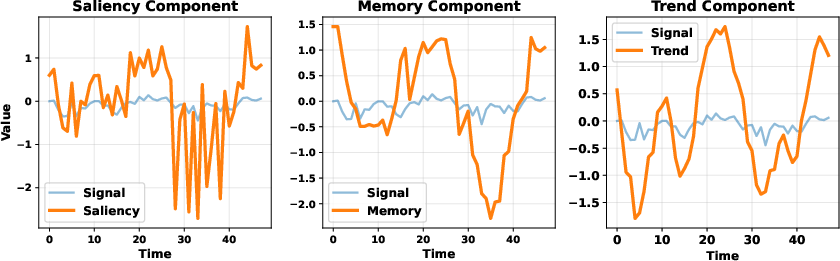
Figure 5: Decomposition on the weather dataset, revealing the relative prominence of the trend component.

Interpretability

Interpretability is operationalized by directly examining the learned component weights ($\alpha$) across datasets. The analysis reveals strong adaptation: for example, in household data, saliency receives the largest weight, whereas trend dominates in weather data.

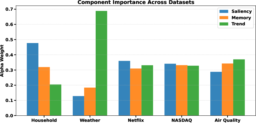
Figure 6: Learned component weights ($\alpha$) across datasets, providing insight into data-dependent temporal modeling.

These weights correspond to explicit hypotheses about what temporal structures drive predictive performance in distinct domains.

Limitations and Boundary Conditions

In highly stochastic domains (Netflix/NASDAQ), the $R^2$ of all methods collapses toward zero. SPaRSe-TIME, while competitive, does not outperform more expressive models like Transformers, as the structural prior (clear separation into low-rank, saliency, and trend) is less applicable.

Theoretical and Practical Implications

SPaRSe-TIME establishes that projection-based structured models are a computationally efficient and interpretable alternative to monolithic sequence architectures. Its computational efficiency (fewest parameters, lowest FLOPs, rapid inference) makes it suitable for deployment at scale and in latency-sensitive environments.

However, the limitations exposed in stochastic and multivariate interactions suggest the decomposition is optimal primarily for structured, moderately stationary, or seasonally variable time series. The explicit, interpretable design yields diagnostic insight—it is clear when and why the approach will succeed or fail.

Further, the modular design of SPaRSe-TIME facilitates future augmentation—more expressive saliency mechanisms, dynamic or nonlinear memory channels, or sophisticated multiscale trend extraction could enhance applicability to nonlinear or interaction-rich regimes.

Future Directions

Research extensions can target several axes:

• Learned saliency powered by higher-order statistics or context modeling.
• Nonlinear, dynamic low-rank representations adapting to time-varying structure.
• Integration with attention mechanisms or graph-based relational modeling for dense, interacting multivariate sequences.
• Multi-resolution trend extraction for compound-seasonality domains.
• Automated selection of decomposition hyperparameters ($S(X)$0, smoothing kernel) via meta-learning.

Conclusion

SPaRSe-TIME provides a principled, interpretable, and efficient framework for time series modeling, with clear empirical strengths in domains characterized by decomposable saliency, memory, and trend elements. While its advantages are diminished in highly stochastic and strongly nonlinear domains, its diagnostic transparency and computational performance establish it as a compelling paradigm for interpretable time series analysis. Future work is needed to bridge the gap between efficiency, interpretability, and the flexible modeling capacity required for more complex time series scenarios (2604.17350).