Elucidating the SNR-t Bias of Diffusion Probabilistic Models
Abstract: Diffusion Probabilistic Models have demonstrated remarkable performance across a wide range of generative tasks. However, we have observed that these models often suffer from a Signal-to-Noise Ratio-timestep (SNR-t) bias. This bias refers to the misalignment between the SNR of the denoising sample and its corresponding timestep during the inference phase. Specifically, during training, the SNR of a sample is strictly coupled with its timestep. However, this correspondence is disrupted during inference, leading to error accumulation and impairing the generation quality. We provide comprehensive empirical evidence and theoretical analysis to substantiate this phenomenon and propose a simple yet effective differential correction method to mitigate the SNR-t bias. Recognizing that diffusion models typically reconstruct low-frequency components before focusing on high-frequency details during the reverse denoising process, we decompose samples into various frequency components and apply differential correction to each component individually. Extensive experiments show that our approach significantly improves the generation quality of various diffusion models (IDDPM, ADM, DDIM, A-DPM, EA-DPM, EDM, PFGM++, and FLUX) on datasets of various resolutions with negligible computational overhead. The code is at https://github.com/AMAP-ML/DCW.


Paper Prompts
Sign up for free to create and run prompts on this paper using GPT-5.
Top Community Prompts
Explain it Like I'm 14
Overview
This paper studies a hidden problem in diffusion models (the AI systems that turn noise into images, sounds, or videos). The authors发现 that during generation these models often get the “noise level” wrong for each step. They call this the SNR–t bias. SNR means “signal-to-noise ratio” (how clear the picture is), and t is the timestep (the step number in the process). If the model thinks it’s at a step with a certain clarity but the actual image is noisier or cleaner than expected, the model makes worse guesses and quality drops. The paper explains why this happens and proposes a simple, training-free fix that improves image quality across many diffusion models.
What questions did the paper ask?
The paper focuses on two simple questions:
- Does a mismatch between the expected noise level (SNR) and the current step (timestep) happen during generation, and how does it hurt quality?
- Can we correct this mismatch without retraining the model, and does that improve results?
How did they study it?
To make this understandable, imagine diffusion like drawing a picture by “unblurring” noise step by step:
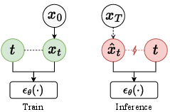
- During training, the model always knows exactly how blurry the image should be at each step.
- During generation, small errors pile up (from the model’s predictions and the math used to step through time). So the image at step t may be a bit more or less blurry than the model expects.
The authors:
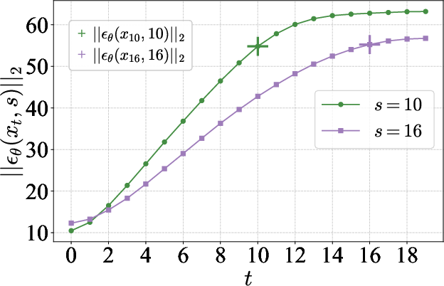
- Measured how the model reacts when it sees images with the “wrong” blur for a given step. They found it tends to over- or under-correct.
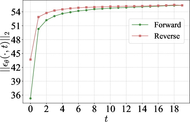
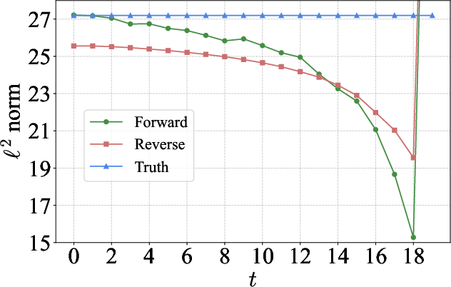
- Showed that, in practice, the image during generation is often noisier (lower SNR) than it should be at each step.
Then they proposed a fix called differential correction:
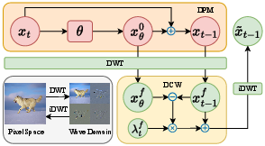
- At each step, diffusion models already produce two things: 1) a “predicted next noisy image,” and 2) a “reconstructed clean image” (their best guess of the final clean picture).
- The authors look at the difference between these two. That difference acts like a gentle nudge pointing the predicted image toward the “right” amount of noise for that step.
- They add a small, controlled amount of this difference back to the predicted image to align its noise level with the step.
To make this even better, they use wavelets:
- Think of an image as having “big shapes” (low-frequency content) and “fine details” like edges and textures (high-frequency content).
- Using a wavelet transform is like splitting a song into bass (low) and treble (high). The authors correct big shapes more at the beginning (when the model focuses on overall structure) and fine details more near the end (when the model adds textures).
- They adjust the strength of these corrections over time, guided by the model’s own noise indicator, so it’s dynamic and stable.
Importantly, this method:
- Requires no retraining.
- Adds almost no extra compute time.
- Works as a plug-in with many diffusion models and samplers.
What did they find?
Here are the main findings and why they matter:
- The mismatch is real and harmful: When the image’s actual SNR doesn’t match the timestep, the model overestimates or underestimates the noise it should remove. This leads to worse images.
- During generation, images are often too noisy for their step: That means the model keeps thinking “it’s clearer than it is,” which causes it to push in the wrong direction and errors accumulate.
- The proposed correction improves quality broadly: Their method consistently improved scores like FID (a standard image quality metric) across many models (IDDPM, ADM, DDIM, A-DPM, EA-DPM, EDM, PFGM++, FLUX) and datasets (from small 32×32 images to larger 256×256 ones).
- For example, on the CIFAR-10 dataset, their plug-in notably lowered FID (better image quality) even with few sampling steps.
- It plays nicely with other fixes: When combined with existing methods that try to reduce “exposure bias” (another kind of mismatch), their approach still adds extra gains.
Why this is important: It shows a root cause (SNR–t mismatch) behind several generation errors and provides a simple, practical fix that works across many systems.
Why this matters
- Better images with less fuss: You get sharper, more accurate pictures (fewer over-smooth or overexposed results) without retraining the model.
- Works widely: Because it’s training-free and plug-and-play, it can be adopted quickly across different diffusion systems.
- A more fundamental understanding: By identifying SNR–t bias as a key issue, the paper gives researchers and engineers a clearer target for improving diffusion models. This could help not just images, but also audio and video generation, where clarity versus noise is just as important.
In short, the paper reveals that diffusion models often get the “blurriness-per-step” wrong during generation, and it offers a simple, clever way to nudge each step back on track—leading to better, cleaner results with minimal extra cost.
Knowledge Gaps
Knowledge gaps, limitations, and open questions
The paper identifies SNR–t bias in diffusion models and proposes a training-free differential correction in the wavelet domain (DCW). Below is a single, concrete list of what remains missing, uncertain, or unexplored:
- Theoretical assumptions are unvalidated: the core reconstruction assumption $\,^0_\theta(\hat{x}_t,t)=\gamma_t x_0+\phi_t\epsilon_t\,$ (Assumption 5.1) is not rigorously derived; the conditions under which and bounds on hold are not characterized, and independence/gaussianity assumptions are not tested empirically.
- “Always lower” reverse-time SNR claim lacks a formal proof: Theorem 5.1 depends on unmeasured and and does not rigorously establish that reverse-time SNR is strictly lower for all , models, and solvers; provide counterexample analysis or sufficient conditions for the inequality to hold.
- No direct estimator for inference-time SNR: experiments use the network’s predicted noise norm as a proxy; a principled, architecture-agnostic SNR estimator (for both VP/VE and continuous-time formulations) is missing, as is calibration of such an estimator against ground truth.
- Unmeasured trajectories: the paper does not extract or fit along the denoising path to quantify bias magnitude, variability across data, and correlation with quality gains; methods to estimate these parameters from model outputs are absent.
- Applicability of the theory to non-DDPM formalisms is unclear: the derivations use DDPM-style ; how the SNR–t bias and the proof translate to EDM, PFGM++, VE/SDE formulations, or ODE-only samplers is not formally established.
- Interaction with numerical solvers and step sizes is underexplored: the dependence of SNR–t bias on solver family (e.g., Euler–Maruyama, Heun, DPM-Solver v3, RK methods), discretization step size, and adaptive-step control is not quantified; links to local truncation error are unexamined.
- Lack of formal stability analysis of DCW: the correction adds a biasing term each step without guarantees on stability, convergence, or error bounds; conditions preventing over-correction, oscillation, or divergence (especially near or at very low NFE) are not provided.
- Limited coverage of extreme regimes: performance and failure modes are not studied for 4–8 steps, >100 steps, near-zero variance regions, or extremely strong/weak noise schedules.
- Unknown impact on likelihoods and calibration: DCW perturbs the reverse process; effects on ELBO/NLL, score consistency, and calibrated likelihoods (where available) are not measured.
- Diversity–fidelity trade-offs are only partially assessed: aside from FID and Recall, impacts on Precision, density/coverage, and (for conditional models) semantic alignment metrics (e.g., CLIP-T) are not reported.
- Conditional generation interactions are unquantified: how DCW behaves under classifier-free guidance (CFG) strength schedules, classifier guidance, or control signals is not analyzed; possible interference with guidance-induced estimates is not studied.
- Scope beyond images is untested: the SNR–t bias and DCW are not evaluated on audio, video, 3D, or other modalities where frequency characteristics and denoising dynamics differ.
- Latent-space pipelines are not addressed: for latent diffusion (e.g., LDMs, SDXL-like), it is unclear whether DCW should act in latent or pixel space, and how the wavelet basis maps to latent representations.
- Content-adaptive weighting is absent: the per-subband coefficients depend only on ; no image-, subband-, or content-adaptive adjustment (e.g., based on local SNR or predicted error) is explored.
- Wavelet design choices are not ablated: number of decomposition levels, wavelet families (Haar, Daubechies, biorthogonal), orientation-specific weighting, and comparisons to alternative transforms (e.g., DCT, steerable pyramids, learned band-pass filters) are missing.
- Potential frequency-domain artifacts are unexamined: ringing, aliasing, or loss of fine texture from repeated DWT/iDWT at each step are not analyzed or quantified.
- Robustness to domain shifts and OOD data is unknown: how SNR–t bias and DCW perform under distribution shifts, corrupted inputs, or style/scene diversity is not reported.
- Negative cases and failure analysis are missing: scenarios where DCW degrades performance (datasets, solvers, guidance strengths, NFEs) are not identified; an error budget attributing gains to bias reduction is not provided.
- Computational scaling is not fully characterized: overhead is measured on modest resolutions; scaling to high-res (e.g., 1024–4K), video, or long trajectories, and memory implications of multi-level transforms are not reported.
- Solver-agnostic error control is unexplored: relating DCW to adaptive error control (e.g., step rejection, embedded methods) or combining it with adaptive timestepping to directly target SNR misalignment is not attempted.
- Formal linkage to exposure bias remains qualitative: although the paper posits SNR–t bias as a root cause, a causal model or controlled experiments that isolate and quantify this relationship are missing.
- Automatic bias detection and correction are not provided: there is no online estimator to detect SNR–t misalignment per step and modulate correction strength accordingly; a closed-loop controller for bias reduction remains an open design.
- Interactions with training-time strategies are unstudied: whether SNR-aware conditioning, curriculum schedules, or training with SNR-mismatched inputs reduces SNR–t bias and how DCW complements or replaces such training is unknown.
- Downstream tasks are not evaluated: effects on image editing, inversion, super-resolution, and controllability (e.g., attention maps) are not explored, despite different sensitivity to frequency components.
- Security and robustness considerations are absent: sensitivity to adversarial perturbations, small changes, or procedural prompts (for T2I) under DCW is not assessed.
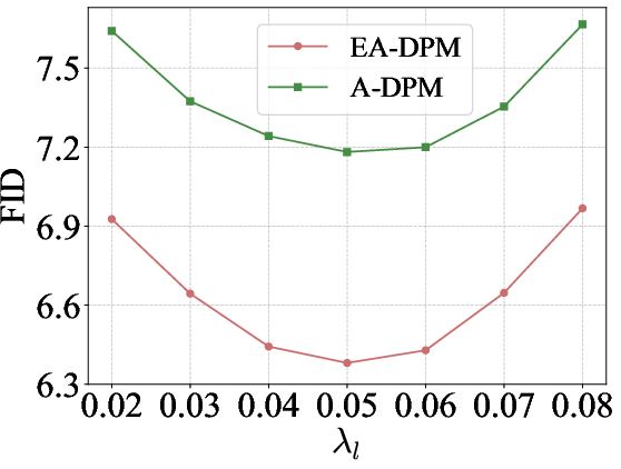
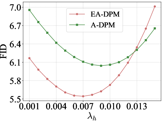
- Parameter selection remains manual: although hyperparameter sensitivity is mild, a principled or learning-based approach to set (e.g., from estimated bias magnitude) is not proposed.
- Quantifying bias–gain correlation is missing: the paper does not measure per-step SNR misalignment and correlate it with improvements from DCW, leaving the causal efficacy partially unsubstantiated.
Practical Applications
Immediate Applications
Below are deployable, concrete ways to use the paper’s findings and the proposed differential correction in wavelet domain (DCW) today.
- Plug-and-play quality boost for diffusion model inference
- What: Wrap existing samplers with DCW to reduce SNR–t bias and improve fidelity/diversity without retraining; gains shown across IDDPM, ADM, DDIM, A‑DPM, EA‑DPM, EDM, PFGM++, DiT, FLUX.
- Sectors: software (ML platforms), media/entertainment (creative tools), advertising, gaming, e‑commerce (asset generation).
- Tools/workflows:
- Add a DCW module between sampler steps (compute x0 reconstruction, DWT/iDWT, apply per-subband correction with σt‑based weights).
- Integrate into PyTorch/HuggingFace Diffusers pipelines, ComfyUI/Stable‑Diffusion UIs as a “SNR correction” toggle.
- Use default λ scheduling from the paper; quick two-stage hyperparameter sweep to tune λl, λh.
- Assumptions/dependencies: inference-time access to model outputs to compute x0 (via epsilon or x0 head), availability of per-step σt, support for DWT/iDWT on latent or pixel space, negligible latency overhead (~0.1–0.5%) acceptable.
- Faster sampling at the same quality (or higher quality at fixed steps)
- What: Use DCW to recover accuracy lost to aggressive step reduction (e.g., EDM/PFGM++/DDIM fast samplers), improving FID substantially at 10–35 NFEs.
- Sectors: online creative generation, ad-tech creatives, real-time UX previews, design iteration.
- Tools/workflows: expose “quality at N steps” presets with DCW; A/B test target FID/recall vs baseline; deploy per‑model DCW configs.
- Assumptions/dependencies: same as above; benefits depend on baseline model and step schedule.
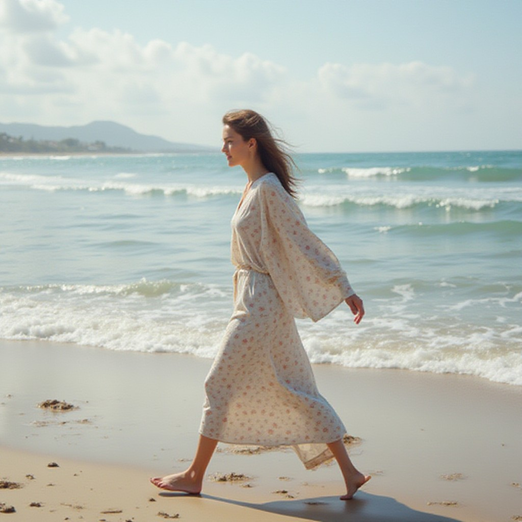
- Text-to-image and image editing artifact reduction
- What: Mitigate over-smoothing/overexposure and improve fine details in models like FLUX and Stable Diffusion.
- Sectors: media/entertainment, prosumer creative apps, social platforms.
- Tools/workflows: inference-side plugin for T2I and editing pipelines; default on for low-step modes; expose per-subband strength sliders to users.
- Assumptions/dependencies: apply DCW in latent space for latent-diffusion models; ensure DWT compatibility with latent dimensionality.
- Synergistic boost for existing exposure-bias mitigations
- What: Stack DCW with ADM‑ES, DPM‑FR, and similar methods to further improve quality.
- Sectors: ML research and model serving providers.
- Tools/workflows: chain DCW after bias-correction samplers; version DCW configs per model.
- Assumptions/dependencies: no retraining required; minor engineering to compose modules.
- Research diagnostics and benchmarking
- What: Use the paper’s SNR–t bias analyses (e.g., compare ||εθ(x,t)|| on forward vs reverse paths) to diagnose sampling schedules and solvers.
- Sectors: academia, applied research labs, model evaluation teams.
- Tools/workflows: add SNR–t alignment plots to training/eval dashboards; monitor bias during distillation or schedule search.
- Assumptions/dependencies: ability to run controlled forward perturbations and log per‑t network outputs.
- Better synthetic data for training downstream models
- What: Use DCW to generate higher-fidelity images for data augmentation (e.g., perception models), reducing texture loss and smoothing.
- Sectors: robotics/autonomy (perception data), retail/product imagery, AR/VR content.
- Tools/workflows: turn on DCW for bulk data synthesis; measure downstream accuracy improvements.
- Assumptions/dependencies: verify distribution shifts are acceptable; revalidate downstream metrics.
- Audio diffusion enhancement (1D adaptation)
- What: Apply differential correction in 1D wavelet or STFT-like domains to improve timbral detail and reduce artifacts in audio DPMs (e.g., DiffWave/WaveGrad).
- Sectors: music/voice generation, podcast tools, audio post-production.
- Tools/workflows: replace 2D DWT with 1D wavelet transform; tune per-band λ.
- Assumptions/dependencies: need per‑step x0 reconstruction and progress metric; hyperparameters must be re-tuned for 1D signals.
- Low-resource and on-device inference upgrades
- What: Improve quality on edge/mobile or cost-constrained servers without retraining or added parameters.
- Sectors: mobile apps, embedded creative tools, edge kiosks.
- Tools/workflows: deploy lightweight DWT kernels; use half-precision where safe; select smaller wavelet bases to minimize overhead.
- Assumptions/dependencies: confirm memory/compute budgets can accommodate small per-step transforms.
- Restoration and super-resolution pipelines
- What: Improve detail integrity in diffusion-based SR and restoration (photo enhancement, deblurring).
- Sectors: media restoration, surveillance, consumer photo apps.
- Tools/workflows: insert DCW into SR samplers; favor higher λ for high-frequency subbands in later steps.
- Assumptions/dependencies: task-specific tuning; confirm that sharpening does not introduce hallucinated artifacts beyond acceptable bounds.
- Remote sensing and geospatial imagery generation/SR
- What: Preserve fine structures (roads, rivers, edges) in diffusion-based upscaling or synthesis of satellite/aerial images.
- Sectors: energy, agriculture, logistics, urban planning.
- Tools/workflows: adapt DCW to multispectral channels; evaluate with task metrics (e.g., edge preservation).
- Assumptions/dependencies: compatible data preprocessing; validate against ground-truth or expert evaluation.
Long-Term Applications
These opportunities may require further research, scaling, validation, or productization.
- SNR-aware training objectives and architectures
- What: Incorporate SNR–t alignment losses, auxiliary heads predicting SNR mismatch, or subband-aware networks to reduce bias during training.
- Sectors: foundational model providers, academia.
- Tools/workflows: new curricula that inject controlled SNR perturbations; joint optimization of solvers and networks.
- Assumptions/dependencies: training cost; ensuring stability and generalization across domains.
- Adaptive solvers that monitor SNR alignment online
- What: Dynamic timestep controllers that adjust step sizes, re-perturb, or tune λ based on measured SNR mismatch during inference.
- Sectors: high-performance inference platforms.
- Tools/workflows: runtime SNR estimators; control policies (e.g., PID/RL) for per-step adaptation.
- Assumptions/dependencies: reliable SNR proxies; minimal additional latency.
- Native wavelet/subband diffusion architectures
- What: Architectures that denoise in wavelet space natively (multi-branch subband U-Nets/Transformers), making DCW implicit.
- Sectors: image/video generation, super-resolution.
- Tools/workflows: training pipelines in wavelet domain; subband-specific losses and schedulers.
- Assumptions/dependencies: stable training; careful design of cross-subband attention.
- Spatiotemporal DCW for video diffusion
- What: Extend differential correction to spatiotemporal wavelets or 3D transforms for video models; maintain temporal consistency while enhancing detail.
- Sectors: film/VFX, advertising, game trailers.
- Tools/workflows: 3D DWT/iDWT or temporal wavelet banks; temporal λ scheduling.
- Assumptions/dependencies: higher compute/memory; need for consistent subband handling across frames.
- Medical imaging reconstruction and synthesis (regulated deployment)
- What: Apply SNR–t bias correction to diffusion-based MR/CT/PET reconstruction/synthesis to improve edge fidelity.
- Sectors: healthcare.
- Tools/workflows: integrate DCW in reconstruction samplers; validate with clinical metrics and reader studies.
- Assumptions/dependencies: rigorous clinical validation, safety/efficacy studies, regulatory approvals; bias and artifact audits.
- Time-series diffusion for finance and energy forecasting
- What: Adapt differential correction to 1D/multivariate diffusion for generating or denoising financial or energy load series using wavelets.
- Sectors: finance, energy.
- Tools/workflows: multiscale 1D wavelet DC; backtesting frameworks to assess calibration and tail behavior.
- Assumptions/dependencies: ensure corrections do not introduce leakage or unrealistic dynamics; domain-specific validation.
- Standardized SNR–t bias metrics and benchmarks
- What: Community benchmarks and reporting standards for SNR alignment curves alongside FID/recall.
- Sectors: academia, industry consortia, regulators.
- Tools/workflows: open datasets and scripts to compute SNR mismatch; model cards including SNR–t metrics.
- Assumptions/dependencies: consensus on proxies/measurement; broad adoption by model hubs.
- Hardware and compiler support for multiresolution inference
- What: Accelerate DWT/iDWT and per-subband operations in inference compilers/accelerators (e.g., TensorRT, TVM, NPUs).
- Sectors: chip vendors, cloud providers, mobile OEMs.
- Tools/workflows: fused kernels for wavelet transforms; memory-efficient tiling for per-step operations.
- Assumptions/dependencies: sufficient demand; co-design with model execution graphs.
- Safety and provenance controls for higher-fidelity generation
- What: As realism increases, integrate watermarking, provenance metadata (C2PA), and misuse detection calibrated for DCW-enhanced outputs.
- Sectors: platforms, publishers, regulators.
- Tools/workflows: post-generation watermarking; classifiers tuned to DCW outputs; policy updates reflecting improved believability.
- Assumptions/dependencies: robust watermark resilience; alignment with platform policies and regulatory requirements.
- Automated hyperparameter tuning and configuration services
- What: Services that learn optimal λ schedules per model/task/dataset, balancing speed/quality.
- Sectors: MLOps, AI platforms.
- Tools/workflows: Bayesian optimization or bandit-based autotuners; deployment of per‑model DCW profiles.
- Assumptions/dependencies: reliable offline metrics correlating with user-perceived quality.
Notes on feasibility across applications:
- The paper’s key assumption for analysis, that x̂0 ≈ γt x0 + φt εt, underpins the theoretical justification of DCW; empirically, results are positive across many models, but edge cases may need tuning.
- DCW requires access to per-step reconstruction x0 and reverse variance σt; most diffusion pipelines can compute these from εθ and schedules.
- Extensions to non-image domains (audio, video, time-series) are promising but need domain-specific transforms and validation.
- While overhead is negligible in reported settings, very low-latency or on-device deployments may require kernel-level optimizations.
Glossary
Below is an alphabetical list of advanced domain-specific terms from the paper, each with a brief definition and a verbatim usage example.
- classifier guidance: A technique that uses a pretrained classifier’s gradients to steer the diffusion sampling process toward desired classes. "ADM employs classifier guidance to make DPMs outperform GANs"
- consistency models: Generative models trained to produce consistent outputs across different noise levels or time steps, enabling fast sampling without iterative denoising. "and consistency models~\cite{song2023consistency,song2024improved,lu2025simplifying,lei2026there} are widely studied."
- deterministic sampling: A sampling regime for diffusion models that removes stochasticity (e.g., via ODE solvers), producing the same output for a fixed input and seed. "In deterministic sampling, we use EDM~\cite{Karras2022edm} and PFGM++~\cite{xu2023pfgm++} as baseline models and measure the sampling cost by Neural Function Evaluations (NFE)~\cite{vahdat2021score}."
- Discrete Wavelet Transform (DWT): A transform that decomposes signals or images into localized frequency components across different scales and orientations. "DCW employs Discrete Wavelet Transform (DWT)~\cite{graps1995introduction} to decompose and into four frequency subbands."
- discretization errors: Numerical inaccuracies introduced when continuous-time dynamics (e.g., SDEs/ODEs) are solved with finite step sizes. "due to network prediction errors and discretization errors in numerical solvers"
- exposure bias: A mismatch between training and inference conditions where a model encounters its own imperfect predictions at test time, compounding errors. "Exposure bias acts across samples, whereas SNR-t bias arises between samples and timesteps."
- frequency subbands: Components obtained by wavelet decomposition that isolate low- and high-frequency content (e.g., ll, lh, hl, hh). "decompose and into four frequency subbands."
- Fréchet Inception Distance (FID): A metric that compares distributions of generated and real images by modeling Inception features with multivariate Gaussians; lower is better. "we employ standard metrics including Fréchet Inception Distance (FID)~\cite{heusel2017gans} and Recall"
- inverse discrete wavelet transform (iDWT): The inverse operation of DWT that reconstructs the signal/image from its subbands. "we utilize the inverse discrete wavelet transform (iDWT)~\cite{graps1995introduction} to map the samples back to the pixel space"
- knowledge distillation: A training paradigm where a smaller or faster “student” model learns to mimic a larger “teacher” model’s behavior. "knowledge distillation-based DPMs~\cite{salimans2022progressive,liu2023instaflow,meng2023distillation,luhman2021knowledge}"
- Markov chains: Stochastic processes where the next state depends only on the current state, used to formalize forward and reverse diffusion processes. "DPMs generally comprise a forward process and a reverse process, with both formulated as Markov chains."
- Neural Function Evaluations (NFE): The number of calls to the neural network during sampling; a proxy for computational cost in diffusion inference. "measure the sampling cost by Neural Function Evaluations (NFE)~\cite{vahdat2021score}."
- numerical solvers: Algorithms (e.g., Euler, Heun, Runge–Kutta) used to approximate solutions of differential equations that govern diffusion sampling. "due to network prediction errors and discretization errors in numerical solvers"
- Ordinary Differential Equation (ODE): A differential equation without stochastic terms used to define deterministic diffusion sampling trajectories. "a numerical solution to a Stochastic Differential Equation (SDE) or an Ordinary Differential Equation (ODE)"
- posterior distribution: The conditional distribution of a latent variable given observations; in diffusion, the distribution of given (and possibly ). "the corresponding posterior distribution can be expressed as:"
- posterior mean: The expected value of the posterior distribution; used as the reconstruction target of in diffusion models. "which is also known as the posterior mean "
- reparameterization: A technique that rewrites random variables to allow gradient-based optimization (e.g., expressing sampling via deterministic functions plus noise). "Through reparameterization, we are able to obtain:"
- reverse process variance (σ_t): The variance term used in the reverse (denoising) transition, indicating uncertainty and often used to modulate sampling dynamics. "the reverse process variance σ_t in DPMs serves as a robust indicator of the denoising progress"
- Signal-to-Noise Ratio (SNR): A measure of signal power relative to noise power; in diffusion, it relates clean and noise components at a given timestep. "the SNR of is directly determined by the timestep :"
- Signal-to-Noise Ratio–timestep (SNR-t) bias: A systematic mismatch during inference between a sample’s actual SNR and the timestep it is conditioned on. "The SNR-t bias refers to the misalignment between the SNR of predicted samples and their assigned timesteps during inference."
- Stochastic Differential Equation (SDE): A differential equation including stochastic (noise) terms, used to define diffusion’s forward and reverse-time dynamics. "a numerical solution to a Stochastic Differential Equation (SDE) or an Ordinary Differential Equation (ODE)"
- stochastic sampling: A sampling regime that includes randomness (e.g., SDE-based solvers), producing different outputs for the same input and seed. "In stochastic sampling, we select A-DPM~\cite{baoanalytic} and NPR-DM in EA-DPM~\cite{bao2022estimating} as the baseline models."
- Tweedie’s formula: A result linking the posterior mean of a signal corrupted by Gaussian noise to the score (gradient of log-density) of the noisy observation. "Based on Tweedie's formula \cite{umdon} and the L2-norm loss function \cite{Karras2022edm}, DPMs tend to predict the mean value of the target data."
- variance schedule: The predefined sequence of noise variances (β_t) used in the forward diffusion process that determines the noising intensity over time. "Given a target data distribution and a variance schedule "
- wavelet domain: A representation space obtained via wavelet transforms where signals are analyzed in localized time–frequency components. "we introduce the method into the wavelet domain, allowing it to correct different frequency components of samples separately."
Collections
Sign up for free to add this paper to one or more collections.