SynthSAEBench: Evaluating Sparse Autoencoders on Scalable Realistic Synthetic Data
Abstract: Improving Sparse Autoencoders (SAEs) requires benchmarks that can precisely validate architectural innovations. However, current SAE benchmarks on LLMs are often too noisy to differentiate architectural improvements, and current synthetic data experiments are too small-scale and unrealistic to provide meaningful comparisons. We introduce SynthSAEBench, a toolkit for generating large-scale synthetic data with realistic feature characteristics including correlation, hierarchy, and superposition, and a standardized benchmark model, SynthSAEBench-16k, enabling direct comparison of SAE architectures. Our benchmark reproduces several previously observed LLM SAE phenomena, including the disconnect between reconstruction and latent quality metrics, poor SAE probing results, and a precision-recall trade-off mediated by L0. We further use our benchmark to identify a new failure mode: Matching Pursuit SAEs exploit superposition noise to improve reconstruction without learning ground-truth features, suggesting that more expressive encoders can easily overfit. SynthSAEBench complements LLM benchmarks by providing ground-truth features and controlled ablations, enabling researchers to precisely diagnose SAE failure modes and validate architectural improvements before scaling to LLMs.

Paper Prompts
Sign up for free to create and run prompts on this paper using GPT-5.
Top Community Prompts
Explain it Like I'm 14
What this paper is about
This paper introduces SynthSAEBench, a tool that creates large, realistic “fake” data so researchers can test and improve a kind of AI tool called a sparse autoencoder (SAE). SAEs are used to break down what big LLMs are thinking into simpler parts called features, so humans can understand them better. Real tests on big models are noisy and confusing, and tiny toy tests are too simple. SynthSAEBench aims to be “just right”: big, realistic, and clear.
The main questions the paper asks
- How can we test different SAE designs fairly and clearly, without the noise and randomness of big LLMs?
- Can we build synthetic (fake but realistic) data that includes the tricky things real models have, like:
- Correlation: related features often happen together
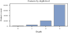
- Hierarchy: big ideas contain smaller ideas (animal → dog → poodle)
- Superposition: many ideas share the same space, so they overlap
- Do results on this synthetic data match things we’ve already seen in real LLMs?
- What new problems can we discover about SAE designs using this setup?
How the researchers built and tested things
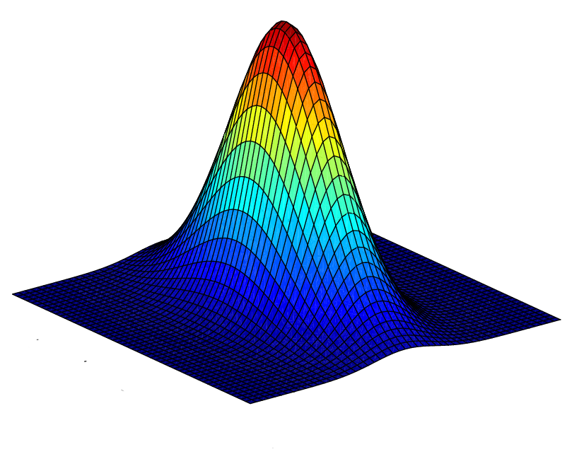
Think of a complex scene like “a golden retriever chasing a ball in a park.” The paper simulates “features” for scenes like this and builds fake hidden activations that look like what a real model might produce.
Here’s the approach, in simple terms:
- Build a dictionary of features
- Imagine a big list of directions, each one pointing to a specific idea (like “dog,” “park,” or “bird”). These are the “true” features in the synthetic world.
- Decide which features are active for a sample
- Correlation: like rolling several “linked” dice, where some dice tend to roll high together. This makes related features occur together (e.g., “dog” and “leash”).
- Hierarchy: a child idea can only appear if its parent does. For example, “poodle” can only appear if “dog” appears.
- Mutual exclusivity: siblings compete; you can’t have two specific breeds of dog in the same single example.
- Set magnitudes
- If a feature is active, how strongly does it show up? The tool gives each active feature a strength.
- Mix features together
- All activated feature directions are added up to make one activation vector, like blending colors to make a final image.
- Make this scalable
- They use math tricks to handle many features efficiently, so the system can scale to tens of thousands of features and still run fast.
How SAEs are evaluated on this synthetic data:
- Reconstruction quality: How well does the SAE rebuild the original activation? (Like redrawing a picture from memory.)
- Feature recovery: How well do the SAE’s learned directions match the “true” features from the synthetic world? They measure this with:
- MCC (Mean Correlation Coefficient): how closely each learned feature matches a true one, using optimal one-to-one matching
- Uniqueness: whether different learned features map to different true features
- Probing (classification): Treat each latent (neuron) like a detector for its best-matching feature and measure precision, recall, and F1.
- Sparsity: L0 is how many latents fire per sample (think “how many switches are on”). They compare this to the ground truth.
They also release a standard test model called SynthSAEBench-16k with:
- 16,384 true features
- Realistic correlation, hierarchy, and superposition
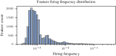
- Zipf-like firing frequencies (few common features, many rare ones)
- Hidden size similar to a real LLM layer
- Clear instructions for training SAEs of width 4096
What they found and why it matters
Here are the key results, written plainly:
- Real behaviors show up in the synthetic world
- The benchmark reproduces patterns seen in real LLM tests:
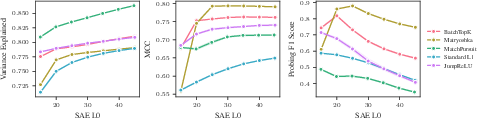
- Matryoshka SAEs: great feature quality but surprisingly worse reconstruction
- Matching Pursuit (MP) SAEs: great reconstruction but poor feature quality
- SAEs do worse than simple supervised probes (like logistic regression) at detecting features
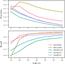
- There’s a trade-off between precision and recall controlled by L0: turning on more latents boosts recall (catch more true features) but hurts precision (more false alarms)
- New problem discovered: MP-SAEs can “overfit” superposition noise
- As features overlap more (more superposition), MP-SAEs get even better at reconstruction but worse at finding the true features. In other words, they learn to fit the messy overlaps instead of the actual underlying ideas. This suggests that more powerful encoders can sometimes chase the wrong thing.
- No current SAE is perfect, even in the best-case world
- This synthetic setup is very friendly to SAEs because the “true” features really are clean straight-line directions. Still, no tested SAE fully discovers the ground-truth features. This points to limits in current SAE designs and training methods.
Why this matters:
- It shows that SAE issues aren’t only caused by real models being messy. Even under ideal conditions, current SAEs struggle.
- The benchmark gives researchers a clear, controlled place to test new ideas and see real improvements before moving to noisy, expensive LLM experiments.
What this could change going forward
- Faster progress: With ground-truth answers and low-noise metrics, researchers can quickly tell if a new SAE idea is actually better.
- Better designs: Understanding failure modes like MP-SAEs overfitting superposition can guide new, smarter architectures.
- Smarter evaluation: Use SynthSAEBench to diagnose problems and tune designs, then confirm on real LLMs.
- Broader science: The authors plan to extend the synthetic world to test other representation ideas beyond simple linear features, like manifolds or soft competition between features.
In short: SynthSAEBench gives the community a realistic, scalable, and trustworthy “wind tunnel” to test SAEs. It explains old puzzles, reveals new ones, and sets a clear target for the next generation of interpretability tools.
Knowledge Gaps
Knowledge gaps, limitations, and open questions
Below is a single, concrete list of what remains missing, uncertain, or unexplored, with actionable directions for future work:
- Transfer validity to LLMs: Quantify how improvements on SynthSAEBench (e.g., MCC, F1, R²) predict gains on SAEBench tasks (sparse probing, autointerp, concept erasure) across architectures and hyperparameters; establish correlation and calibration curves.
- Sensitivity to synthetic model parameters: Systematically ablate Zipf exponent and range, firing magnitude distributions (, ), hierarchy depth/branching/mutual exclusion strength, and correlation rank /scale ; report robustness of conclusions under these changes.
- Realism of co-firing structure: Validate the Gaussian copula against empirical LLM feature co-occurrence (including tail dependence and negative correlations); compare alternative copulas (e.g., t-copula, vine copulas) and fit parameters to measured LLM statistics.
- Superposition characterization: Go beyond mean max cosine () by measuring mutual coherence, the spectrum of , and overlap distributions; relate these to SAE failure modes and performance.
- Hierarchy generality: Extend from tree structures with hard mutual exclusion to DAGs, multi-parent relations, and soft mutual exclusion (e.g., softmax-based) and evaluate how Matryoshka and other SAEs behave under these regimes.
- Decoder bias effects: Ablate the presence and magnitude of the bias vector (e.g., ); quantify its impact on reconstruction, latent purity, and whether it induces spurious features.
- Scaling laws for training: Derive compute–quality tradeoffs by varying SAE width, depth (stacked/nested SAEs), number of training samples, batch size, optimizer, and learning rate; compare across architectures.
- Sparsity control methods: Compare the L0 controller to alternatives (annealing, per-latent penalties, target sparsity distributions) and quantify effects on precision–recall and MCC.
- MP-SAE overfitting mechanism: Diagnose how MP-SAEs exploit superposition; test regularizers (decoder orthogonality, residual penalties), modified selection rules, early stopping variants, and noise-injection; develop training-time diagnostics to detect this failure mode.
- JumpReLU vs BatchTopK discrepancy: Investigate the observed JumpReLU underperformance at high L0 via analysis of encoder/decoder gradients, activation statistics, bias tying, and architectural tweaks (e.g., skip connections).
- Metrics for known pathologies: Add targeted measures for absorption, splitting, and hedging (e.g., parent–child alignment scores, correlation leakage indices, per-feature AUROC/PR curves) beyond MCC/F1/R²/uniqueness/dead latents.
- Matching assumptions: Relax one-to-one Hungarian matching to evaluate many-to-one (mixtures) and quantify coverage vs purity; report both coverage (fraction of ground-truth features represented) and purity (per-latent specificity).
- Generalization and distribution shift: Specify train/test splits and evaluate overfitting; test robustness to shifts in firing probabilities, correlation, and hierarchy; calibrate latent thresholds and measure metric stability under shifts.
- Interaction ablations: Jointly vary pairs of phenomena (e.g., high correlation with deep hierarchy, or strong superposition with tight mutual exclusion) to map regimes of success/failure for each architecture.
- Coefficient and nonlinearity realism: Explore heavy-tailed, skewed, signed coefficients and non-ReLU generative nonlinearities (e.g., GELU-like) to better mirror LLM activations; assess SAE performance under these distributions.
- Sequence/context dynamics: Extend the synthetic model to token- and position-conditioned features, attention-induced dependencies, and temporal correlations to capture transformer sequence effects.
- Cross-model/layer realism: Validate the benchmark against activation statistics from multiple LLMs and layers (vary , mean/stdev norms) to ensure conclusions are not tied to Pythia-160m layer 10.
- Fair comparison practices: Tune each architecture with best-known settings (e.g., MP early stopping variants, Matryoshka auxiliary losses to prevent dead latents) and report sensitivity analyses to ensure fairness.
- Reproducibility and versioning: Provide seeds, parameter dumps, generation hashes, metric implementations, and benchmark versioning; quantify metric noise (stdevs) across seeds and runs to enable cross-lab comparability.
- Theoretical guarantees: Develop identifiability and error bounds linking LRH properties (coherence, correlation, hierarchy) to recoverability for different SAE architectures under SynthSAEBench regimes.
- Safe encoder expressivity: Determine constraints (e.g., monotonicity, Lipschitz bounds, sparsity priors) that allow more expressive encoders to avoid overfitting superposition noise while improving feature recovery.
- Closing the probe gap: Explore hybrid architectures/losses (e.g., supervised auxiliary signals, sparse probes coupled to decoders) that approach logistic regression probe performance while maintaining sparsity and interpretability.
- Metric aggregation for usefulness: Define composite scores that predict downstream interpretability outcomes (autointerp quality, concept erasure efficacy) and validate their predictive power on LLM tasks.
- Rare feature recovery: Quantify recovery rates across the Zipf tail; test reweighting, curricula, or importance sampling to improve learning of rare features without degrading common-feature performance.
- Dead latent mitigation: Develop principled methods to prevent and detect dead latents across architectures (e.g., adaptive firing targets, diversity losses) while avoiding feature duplication.
Glossary
- Auxiliary loss: An additional term in the training objective used to encourage desirable properties (e.g., ensuring latents fire). Example: "There is sometimes also an additional auxiliary loss with coefficient to ensure all latents fire."
- BatchTopK (BTK): A nonlinearity/selection mechanism that activates the top-k latents across a batch, enforcing sparsity without an explicit penalty. Example: "TopK \citep{gao2024scaling} or BatchTopK (BTK) \citep{bussmann2024batchtopk}."
- Bernoulli-Gaussian model: A generative model where sparse binary indicators (Bernoulli) gate continuous magnitudes (Gaussian), common in dictionary learning. Example: "Our synthetic data model extends the traditional bernoulli-gaussian model commonly used in dictionary learning literature~\citep{Gribonval2010Dictionary,wang2020unique}"
- Bipartite matching: An optimization to find the best one-to-one alignment between two sets (e.g., learned and ground-truth features). Example: "using optimal bipartite matching."
- Dead latents: Latent units that never activate, indicating wasted capacity or training issues. Example: "Dead latents represent wasted capacity and indicate training issues."
- Decoder bias: A learned bias vector added to reconstructions in the decoder of an autoencoder. Example: "a decoder , a decoder bias "
- Dictionary learning: Learning a set of basis vectors (“dictionary”) that can sparsely represent data. Example: "to recover underlying feature directions via sparse dictionary learning."
- Explained Variance (): A reconstruction metric measuring how much variance in inputs is captured by reconstructions. Example: "Explained Variance ()."
- Feature absorption: A failure mode where broader features absorb more specific ones in hierarchical settings. Example: "leading to phenomena like feature absorption \citep{chanin2025a}."
- Feature hedging: A failure mode where latents represent mixtures of correlated features rather than clean concepts. Example: "leading to phenomena like feature hedging \citep{chanin2025feature,chanin2025sparse}."
- Feature Hierarchy: Structural dependencies where specific features can only activate when their more general parent features are active. Example: "Feature Hierarchy"
- Folded normal distribution: The distribution of the absolute value of a normal random variable, used here for heterogeneous magnitude variances. Example: "folded normal distributions: ."
- Gaussian copula: A method to generate correlated binary indicators by thresholding samples from a multivariate normal with a chosen correlation structure. Example: "using a Gaussian copula approach to generate correlated binary firing indicators."
- Ground-truth features: The true, known feature directions and activations used to generate synthetic data, enabling precise evaluation. Example: "providing ground-truth features and controlled ablations"
- Hungarian algorithm: A polynomial-time algorithm for optimal assignment in bipartite graphs, used to match learned latents to true features. Example: "via the Hungarian algorithm"
- JumpReLU: A modified ReLU-like nonlinearity used in SAEs aimed at improving reconstruction fidelity. Example: "typically ReLU or a variant like JumpReLU \citep{rajamanoharan2024jumping}"
- Latent: A hidden neuron/unit in the SAE’s internal representation capturing a feature. Example: "hidden neurons, called ``latents''."
- Linear Representation Hypothesis (LRH): The hypothesis that concepts are represented as (nearly orthogonal) linear directions in activation space. Example: "The Linear Representation Hypothesis (LRH) \citep{park2024lrh} posits that concepts (hereafter ``features'') are represented as nearly-orthogonal linear directions."
- L0 (L-zero): The count of nonzero activations (number of active latents), used as a sparsity measure. Example: "a precision-recall trade-off mediated by L0."
- L1 norm: The sum of absolute values, used as a sparsity penalty encouraging many coefficients to be exactly zero. Example: "For standard L1 SAEs, is the L1 norm of ."
- Low-rank correlation matrix: A correlation structure approximated by a low-rank factorization to model dependencies efficiently at scale. Example: "We support randomly generating a low-rank correlation matrix for use in the synthetic model."
- Matching Pursuit (MP) SAE: An SAE variant that greedily selects latents serially by their projection onto the current residual, without an explicit encoder. Example: "A Matching Pursuit (MP) SAE \citep{costa2025flat} acts like a TopK SAE where the latents are selected in serial rather than in parallel."
- Matryoshka SAE: An SAE variant trained with nested prefix losses so that early latents capture more general features. Example: "A matryoshka SAE \citep{bussmann2025learning} extends the SAE definition by summing losses created by prefixes of SAE latents."
- Mean Correlation Coefficient (MCC): A feature-recovery metric computed by optimally matching learned and true features and averaging their absolute cosine similarities. Example: "Mean Correlation Coefficient (MCC)."
- Mutual exclusion: A constraint in hierarchical features where sibling features cannot be active simultaneously. Example: "we support mutual exclusion among siblings"
- Orthogonalization procedure: An optimization step that reduces pairwise cosine similarities among feature vectors to limit spurious correlations. Example: "we optionally apply an orthogonalization procedure to minimize pairwise cosine similarity."
- Precision-recall trade-off: The inverse relationship between precision and recall observed as sparsity changes, here controlled by L0. Example: "demonstrating the precision-recall trade-off mediated by SAE L0"
- Rectified Gaussian: A nonnegative magnitude distribution obtained by applying ReLU to Gaussian samples for active features. Example: "coefficients are sampled from a rectified Gaussian distribution:"
- Sparse autoencoder (SAE): An autoencoder trained to produce sparse latent representations that aim to align with underlying features. Example: "Sparse autoencoders (SAEs)."
- Superposition: The representation of more features than dimensions by using non-orthogonal directions that overlap in the same space. Example: "a phenomenon known as superposition~\citep{elhage2022toy}."
- TopK: A sparsity-inducing nonlinearity that keeps only the k largest activations per sample. Example: "TopK \citep{gao2024scaling}"
- Zipfian distribution: A heavy-tailed distribution where probability decays as a power law with rank, used for feature firing probabilities. Example: "we use a Zipfian distribution as our default"
Practical Applications
Immediate Applications
Below are applications that can be deployed now using the SynthSAEBench toolkit, benchmark model (SynthSAEBench-16k), and the evaluation methodology presented in the paper.
- Industry/Software: SAE architecture bake-off and rapid prototyping
- Use SynthSAEBench-16k to compare SAE variants (L1, BatchTopK, Matryoshka, JumpReLU, Matching Pursuit) under controlled, low-noise metrics (MCC, F1, R²), before scaling to LLMs.
- Tools/Workflows: SAELens extension + Hugging Face model; automated experiment scripts; MCC/Hungarian matching; precision/recall monitoring by L0.
- Assumptions/Dependencies: LRH-style linear features; access to a single modern GPU (H100 or smaller with fewer samples); transferability of results to real LLM settings is partial.
- AI Safety and Reliability: Failure-mode detection suite for encoders
- Stress-test encoders (e.g., MP-SAEs) against controlled superposition levels to identify overfitting-on-noise behaviors that inflate reconstruction but degrade feature recovery.
- Tools/Workflows: “Superposition stress-test” using variable hidden dimension; dashboards highlighting divergence between R² and MCC/F1.
- Assumptions/Dependencies: Synthetic superposition approximates real model overlap; mapping superposition levels to LLM layers requires domain calibration.
- MLOps: Interpretability CI gate for model releases
- Integrate SynthSAEBench tests into CI/CD to require SAE improvements clear predefined thresholds (e.g., MCC/F1 at target L0) before deployment into LLM interpretability pipelines.
- Sectors: Finance, healthcare, gov-tech (high-stakes compliance environments).
- Tools/Workflows: Nightly CI jobs; standardized metrics report (MCC, uniqueness, dead latents); regression tests across seeds to minimize noise.
- Assumptions/Dependencies: Organizational buy-in; acceptance that synthetic performance is a proxy for likely LLM behavior.
- Engineering: L0 auto-tuning controller adoption
- Apply the paper’s L0 controller to standard L1 and JumpReLU SAEs to hit desired sparsity targets that mediate precision-recall trade-offs aligned with task needs (e.g., higher recall for anomaly detection, higher precision for compliance).
- Sectors: Moderation, fraud detection, content filtering.
- Tools/Workflows: Controller API; scheduled sparsity coefficient adjustments; per-task L0 policies.
- Assumptions/Dependencies: Target L0 generalizes from synthetic to in-domain distributions; tasks tolerate the documented precision-recall trade-off.
- Model Governance: Probe-vs-SAE selection policy
- Adopt logistic regression probes in cases where classification F1 is paramount (paper shows probes beat SAEs decisively), and reserve SAEs for representation analysis/latent discovery.
- Sectors: Compliance reporting (finance/health), risk scoring, content policy audits.
- Tools/Workflows: Side-by-side probe vs SAE evaluation; F1/precision/recall monitoring; documented decision criteria.
- Assumptions/Dependencies: Features of interest behave similarly to synthetic ground-truth signals; labeled data for probes is available.
- Academic Teaching and Training: Hands-on interpretability lab
- Use the synthetic generator (correlation, hierarchy, mutual exclusion, Zipfian firing) to teach superposition and sparsity effects, and reproduce known LLM SAE phenomena in low-noise settings.
- Sectors: Education, research training programs.
- Tools/Workflows: Classroom labs; controlled ablations; assignments comparing Matryoshka vs. MP-SAEs and precision-recall by L0.
- Assumptions/Dependencies: LRH holds in the teaching context; compute availability (can downscale features).
- R&D: Ablation-driven loss and architecture design
- Prototype new encoder/decoder structures and auxiliary losses against ground-truth metrics to diagnose absorption, hedging, and dead-latent issues quickly.
- Tools/Workflows: SynthSAEBench API; hierarchical gating; low-rank correlation; MCC/uniqueness trace during training.
- Assumptions/Dependencies: Synthetic findings guide real-world improvements; careful transfer studies still required.
- AI Tooling: Latent quality and sparsity dashboard
- Ship a productized dashboard that tracks MCC, uniqueness, dead latents, L0 alignment with ground truth, and the reconstruction-vs-quality disconnect for teams iterating on SAEs.
- Sectors: AI platform vendors, enterprise ML teams.
- Tools/Workflows: Metric collectors; seed stability reports; template visualizations.
- Assumptions/Dependencies: Teams instrument their training loops; access to evaluation activations.
Long-Term Applications
Below are applications that will require further research, scaling, or development to reach production-grade maturity.
- Standards and Certification: Industry-wide interpretability benchmarks
- Establish SynthSAEBench-like suites (with versioning) as pre-deployment certifications for interpretability tooling, complementing LLM-based SAEBench with low-noise synthetic tests.
- Sectors: Policy, standards bodies, regulated industries.
- Tools/Workflows: Benchmark registry; pass/fail criteria; audit trails; reproducibility packs.
- Assumptions/Dependencies: Cross-organizational consensus; maintaining relevance across evolving model classes.
- Robust Encoder Design: Superposition-aware SAE architectures
- Develop encoders that retain reconstruction but do not overfit noise, improving MCC/F1 under high superposition; could include constraints, regularizers, or selection mechanisms beyond MP.
- Sectors: AI safety, foundation model providers.
- Tools/Workflows: New encoder families; superposition diagnostics; controlled training curricula.
- Assumptions/Dependencies: Success depends on bridging synthetic to LLM transfer; new theory and empirical validation required.
- Training-time Interpretability Constraints
- Integrate Matryoshka-like losses or sparsity controllers directly into foundation model training to structure feature hierarchies and monosemanticity for downstream transparency and steering.
- Sectors: Foundation models, enterprise AI platforms.
- Tools/Workflows: Joint training recipes; multi-stage curricula; monitoring of latent quality during pretraining.
- Assumptions/Dependencies: Compute overhead; impact on downstream performance; stability of constraints in large-scale training.
- Sector-specific interpretable systems (healthcare, finance, robotics)
- Tailor synthetic generators to domain-specific hierarchies/correlations (e.g., medical ontologies, product taxonomies) to pressure-test interpretability methods before application to sensitive models.
- Tools/Workflows: Domain-specific dictionaries; hierarchy/mutual exclusion modeling; task-aligned L0 targets.
- Assumptions/Dependencies: Availability of domain knowledge; mapping synthetic to real-world tasks; regulatory acceptance.
- Regulatory Compliance Metrics for Explainability
- Adapt MCC/uniqueness and precision/recall-by-L0 into explainability scorecards for audits, impact assessments, and procurement policies.
- Sectors: Finance, healthcare, public-sector AI.
- Tools/Workflows: Compliance dashboards; external audit packs; benchmark notarization.
- Assumptions/Dependencies: Regulators accept synthetic surrogates; alignment with legal definitions of explainability.
- Extensions beyond LRH: Minkowski and manifold-based synthetic benchmarks
- Build next-generation synthetic frameworks modeling polytopes (Minkowski Representation Hypothesis) or feature manifolds; evaluate whether SAE variants generalize beyond linear directions.
- Sectors: Advanced ML research; safety-critical AI.
- Tools/Workflows: New generators; evaluation metrics for manifolds; encoder/decoder redesign.
- Assumptions/Dependencies: New theory, scalable implementations, and metrics that retain low variance.
- Model Auditing Pipelines: Superposition-aware risk assessment
- Incorporate superposition profiling into audits of LLM layers, using synthetic calibration to flag layers where interpretability methods are likely to overfit or yield poor latent quality.
- Sectors: AI assurance providers; internal risk teams.
- Tools/Workflows: Layerwise superposition estimation; audit reports linking reconstruction to feature recovery risks.
- Assumptions/Dependencies: Reliable superposition estimation on real models; accepted risk frameworks.
- Real-time Steering and Safety Mechanisms
- Deploy improved SAEs (post-robustness research) for feature-level steering in production LLMs, enabling safer outputs in moderation, copilots, and autonomous agents.
- Sectors: Software, robotics, education tech.
- Tools/Workflows: Latent steering APIs; runtime monitoring of precision/recall; guardrail integration.
- Assumptions/Dependencies: SAE quality approaches probe-level F1; integration overhead and latency budgets.
Cross-cutting assumptions and dependencies
- The synthetic framework assumes LRH (features are linear directions). External validity to LLMs is strong for phenomena reproduction but not guaranteed for all tasks.
- Compute availability is a practical constraint; results can be downscaled (fewer features/samples) with some loss of fidelity.
- Organizational adoption depends on accepting synthetic benchmarks as a complement to, not a replacement for, LLM-based tests.
- Domain-specific adaptation (hierarchies, correlations, firing distributions) is needed for sector deployments to reflect real concept structures.
Collections
Sign up for free to add this paper to one or more collections.