Balancing Frequencies and Pixels in Flow Matching

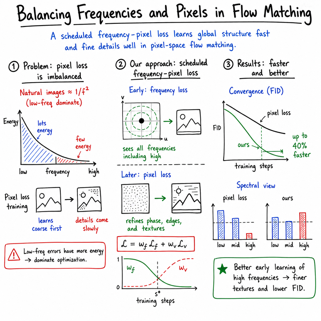
Abstract: Natural images follow a $1/f^2$ spectral distribution: most signal energy lies in the low spatial frequencies, while the perceptually important structures such as textures and edges occupy sparse high-frequency bands. Pixel-space reconstruction objectives, however, treat all spatial errors uniformly, causing low frequencies to dominate the optimization signal and delaying the learning of fine-scale details. In this work, we identify this objective-level spectral imbalance as a key inefficiency in training pixel-space flow models. To address it, we propose a Focal Log-Frequency Loss (f-loss), a spectrally balanced objective that equalizes the learning signal across frequencies, emphasizing high-frequency components that are otherwise underrepresented in pixel-space objectives. Building on this, we introduce a simple training strategy that combines frequency and pixel supervision: we first emphasize frequency-domain learning early to capture all frequencies, and then transition to standard pixel-space v-loss for spatial refinement. This balancing mitigates the low-frequency bias of pixel losses and aligns the training signal with the evolving needs of the model. Our approach is conceptually simple, requires no architectural changes, and acts as a drop-in replacement for flow matching losses. Across multiple model scales, it accelerates convergence by up to 40% while consistently improving FID and perceptual fidelity. We will release code and models.

• The paper identifies an imbalance issue in pixel-space flow-matching models. Low-frequency components disproportionately dominate training because of the spectral characteristics of natural images, leading to suboptimal high-frequency structure recovery.
• The proposed Focal Log-Frequency Loss introduces adaptive logarithmic weighting to target specific spectral components effectively. This loss contributes to balancing frequency components during early training stages and improves overall perceptual detail.
• The experimental findings demonstrate improved convergence and generation quality, showing that adaptive frequency supervision – especially when used early in training – provides significant performance gains and mitigates the imbalance in spectral learning.
• Find recent papers on [frequency modulation in image generation algorithms].

Problem formulation and central claim

"Balancing Frequencies and Pixels in Flow Matching" (2609.02748) examines an optimization pathology in pixel-space flow-matching models: standard spatial regression objectives allocate disproportionate training signal to low spatial frequencies. The paper attributes this imbalance to the spectral statistics of natural images, whose power spectra approximately follow a $1/f^2$ law. Low-frequency components therefore carry substantially more energy than high-frequency components, while edges, textures, and other perceptually consequential structures are concentrated in sparse high-frequency bands.

The resulting mismatch is between numerical reconstruction error and perceptual importance. A pixel-space squared-error objective weights residuals according to their spatial-domain magnitude. Since low-frequency residuals are typically larger, they dominate the gradients during early optimization. The model consequently learns global structure before fine-scale detail, and the paper argues that this is not merely a benign ordering of learning: the early low-frequency bias can impair the eventual recovery of high-frequency content.

The study focuses on pixel-space flow matching in the JiT framework, where direct velocity prediction is reformulated as $x$-prediction. For the linear interpolant

$x_t=(1-t)\epsilon+t x_1,$

the velocity target can be written as

$v^* = x_1-\epsilon=\frac{x_1-x_t}{1-t}.$

If the network predicts $x_\theta$, the conventional velocity objective becomes a timestep-weighted reconstruction loss on the clean image:

$$\mathcal{L}_v = \mathbb{E} \left[ \frac{1}{(1-t)^2} \left\|x_\theta(x_t,t)-x_1\right\|^2 \right].$$

This parameterization is important to the paper’s experimental setting. The authors do not primarily propose a new architecture or transport path; instead, they modify the objective used to train an existing pixel-space flow model.

Spectral diagnosis of pixel-space training

The empirical diagnosis has two components. First, the authors measure the radially averaged power spectrum of images generated by a model trained with the conventional pixel-space objective and compare it with that of real ImageNet images. During training, the model overestimates low and mid frequencies, particularly below approximately $10^{-1}$ cycles per pixel. At high frequencies, especially above approximately $8\times10^{-1}$ cycles per pixel, the generated spectrum is increasingly deficient, with the discrepancy approaching $-60\%$ near the Nyquist limit.

This result establishes that the bias is observable at the level of generated distributions rather than only in per-example reconstruction residuals. The implication is that a model can achieve substantial pixel-space progress while retaining a systematic spectral distortion that suppresses perceptually important texture and edge statistics.

Second, the authors construct a controlled toy problem in which an MLP must reproduce a signal containing exactly two spatial frequencies: one low and one high. The low-frequency component is learned rapidly, whereas the high-frequency component remains substantially underrepresented throughout training. This experiment isolates the temporal learning asymmetry from the complexities of ImageNet and transformer architectures.

Figure 1: In the two-frequency toy experiment, the low-frequency component is learned rapidly while the high-frequency component remains poorly recovered throughout optimization.

The toy result supports the paper’s stronger interpretation of spectral bias: the issue is not simply that high frequencies require more iterations; early optimization may shape the model’s representational allocation in a way that makes later recovery incomplete. The authors nevertheless identify the origin of this effect as an open question. Their experiments demonstrate the phenomenon and its consequences, but do not derive a complete mechanistic account connecting the data spectrum, network architecture, gradient geometry, and irreversible capacity allocation.

Focal Log-Frequency Loss

The proposed frequency-domain objective, referred to in the manuscript as the Focal Log-Frequency Loss, operates on the 2D discrete Fourier transform of the prediction and target. Let the per-frequency residual magnitude be

$$e_{u,v} = \left| \mathcal{F}_{\mathrm{pred}}(u,v) - \mathcal{F}_{\mathrm{target}}(u,v) \right|.$$

The loss combines three design elements.

First, it retains the conventional timestep factor $x$0. This preserves the weighting induced by the $x$1-prediction reformulation rather than introducing a new temporal training distribution.

Second, it uses a focal coefficient based on the residual at each frequency, normalized by the maximum residual in the sample. The normalization is stop-gradient and therefore functions as a data-dependent coefficient rather than an additional differentiable pathway. This emphasizes relatively difficult spectral components while reducing variation in loss scale across examples.

Third, it applies logarithmic compression to the residual magnitude through $x$2. This prevents a small number of large spectral residuals from monopolizing the objective. The authors interpret the operation as a continuous analogue of a Laplacian-pyramid decomposition: logarithmic compression assigns comparable importance across successive frequency scales instead of allowing high-energy low-frequency bands to dominate.

The conceptual claim is therefore more specific than simply “adding a Fourier loss.” The objective attempts to balance individual frequencies while preserving residual adaptivity. The ablations support the necessity of both components. The original focal frequency loss performs poorly, with guided FID of $x$3, whereas the proposed normalized and logarithmically compressed formulation reaches guided FID $x$4 in the corresponding B-size experiment. A logarithmic transformation without the complete normalization scheme improves performance but remains inferior to the full formulation, which achieves unguided FID $x$5 and guided FID $x$6.

The continuous formulation also outperforms coarse spectral partitioning. Discrete decompositions improve as the number of frequency-orientation cells increases: guided FID declines from $x$7 for $x$8 cells to $x$9 for $x_t=(1-t)\epsilon+t x_1,$0 cells, while the continuous formulation reaches $x_t=(1-t)\epsilon+t x_1,$1. This trend is consistent with the paper’s argument that a fine-grained spectral weighting is preferable to a small number of manually selected bands.

Scheduled combination of spectral and pixel supervision

Although the frequency loss accelerates early spectral learning, the paper finds that it plateaus when used alone. The authors attribute this to the loss’s limited sensitivity to Fourier phase. Magnitude alignment can improve the distribution of spectral energy without uniquely specifying the spatial locations of edges and textures. Pixel supervision, by contrast, directly constrains phase and local spatial coherence.

This motivates the scheduled joint objective

$x_t=(1-t)\epsilon+t x_1,$2

where $x_t=(1-t)\epsilon+t x_1,$3 follows a decreasing sigmoid schedule and $x_t=(1-t)\epsilon+t x_1,$4. Frequency supervision dominates at the beginning of training and pixel supervision dominates after the empirically determined crossover point. The switch point is selected using the intersection of validation FID curves for the two component losses, rather than through an extensive grid search. It occurs at approximately 200k steps for B and L models and approximately 350k steps for XL models.

The schedule is not an arbitrary interpolation. It encodes a stage-dependent division of labor: frequency supervision addresses the early spectral bottleneck, whereas pixel supervision provides late-stage phase and spatial refinement. The ablation is especially informative because a reversed schedule performs among the worst configurations. In the B-size guided experiment, the proposed schedule reaches FID $x_t=(1-t)\epsilon+t x_1,$5 at epoch 80, $x_t=(1-t)\epsilon+t x_1,$6 at epoch 200, and $x_t=(1-t)\epsilon+t x_1,$7 at epoch 320. Reversing the schedule produces FIDs $x_t=(1-t)\epsilon+t x_1,$8, $x_t=(1-t)\epsilon+t x_1,$9, and $v^* = x_1-\epsilon=\frac{x_1-x_t}{1-t}.$0, respectively. Thus, the ordering of supervision matters; merely combining the two objectives is insufficient.

Figure 2: The scheduled frequency–pixel objective improves convergence relative to the conventional pixel-space objective while preserving the late-stage refinement advantages of pixel supervision.

The frequency-band analysis directly supports this interpretation. At early training checkpoints, the scheduled objective reduces both low- and high-frequency magnitude errors faster than either component alone. By 400k steps, it reaches low-frequency error approximately $v^* = x_1-\epsilon=\frac{x_1-x_t}{1-t}.$1 and high-frequency error approximately $v^* = x_1-\epsilon=\frac{x_1-x_t}{1-t}.$2, compared with $v^* = x_1-\epsilon=\frac{x_1-x_t}{1-t}.$3 and $v^* = x_1-\epsilon=\frac{x_1-x_t}{1-t}.$4 for the pixel loss and $v^* = x_1-\epsilon=\frac{x_1-x_t}{1-t}.$5 and $v^* = x_1-\epsilon=\frac{x_1-x_t}{1-t}.$6 for the frequency loss. The scheduled loss therefore combines early spectral alignment with late spatial refinement rather than optimizing one frequency regime at the expense of another.

Experimental design

Experiments use class-conditional ImageNet at $v^* = x_1-\epsilon=\frac{x_1-x_t}{1-t}.$7 and $v^* = x_1-\epsilon=\frac{x_1-x_t}{1-t}.$8 resolution. The primary backbone is JiT with B, L, and XL model scales. Training conditions are held fixed across objectives: batch size 1024, AdamW, learning rate $v^* = x_1-\epsilon=\frac{x_1-x_t}{1-t}.$9 after five warmup epochs, no weight decay, and exponential moving average with decay $x_\theta$0. Sampling uses 50 Heun ODE steps, and evaluation is based on 50k generated samples. The authors report FID as the principal metric and additionally use FDD and IS in ablations.

This controlled setup is a strength because it isolates loss-level effects from architectural changes. The paper also evaluates PixelDiT, demonstrating that the method is not restricted to the JiT implementation. However, the principal evidence remains concentrated on ImageNet class-conditional generation and a small number of pixel-space transformer families.

Convergence and generation quality

Across model sizes, the scheduled objective consistently improves FID from the earliest reported checkpoints. At $x_\theta$1, the guided FID at epoch 80 improves from $x_\theta$2 to $x_\theta$3 for JiT-B/16, from $x_\theta$4 to $x_\theta$5 for JiT-L/16, and from $x_\theta$6 to $x_\theta$7 for JiT-XL/16. At later checkpoints, the advantage persists: at epoch 320, guided FID is $x_\theta$8, $x_\theta$9, and $$\mathcal{L}_v = \mathbb{E} \left[ \frac{1}{(1-t)^2} \left\|x_\theta(x_t,t)-x_1\right\|^2 \right].$$0 for B, L, and XL, respectively, compared with $$\mathcal{L}_v = \mathbb{E} \left[ \frac{1}{(1-t)^2} \left\|x_\theta(x_t,t)-x_1\right\|^2 \right].$$1, $$\mathcal{L}_v = \mathbb{E} \left[ \frac{1}{(1-t)^2} \left\|x_\theta(x_t,t)-x_1\right\|^2 \right].$$2, and $$\mathcal{L}_v = \mathbb{E} \left[ \frac{1}{(1-t)^2} \left\|x_\theta(x_t,t)-x_1\right\|^2 \right].$$3 for the pixel-space baseline.

At $$\mathcal{L}_v = \mathbb{E} \left[ \frac{1}{(1-t)^2} \left\|x_\theta(x_t,t)-x_1\right\|^2 \right].$$4, the improvement is similarly pronounced at early training. For JiT-B/32, guided FID at epoch 80 decreases from $$\mathcal{L}_v = \mathbb{E} \left[ \frac{1}{(1-t)^2} \left\|x_\theta(x_t,t)-x_1\right\|^2 \right].$$5 to $$\mathcal{L}_v = \mathbb{E} \left[ \frac{1}{(1-t)^2} \left\|x_\theta(x_t,t)-x_1\right\|^2 \right].$$66.41$$\mathcal{L}_v = \mathbb{E} \left[ \frac{1}{(1-t)^2} \left\|x_\theta(x_t,t)-x_1\right\|^2 \right].$$74.58. By epoch 320, the corresponding values are $$\mathcal{L}_v = \mathbb{E} \left[ \frac{1}{(1-t)^2} \left\|x_\theta(x_t,t)-x_1\right\|^2 \right].$$8 and $$\mathcal{L}_v = \mathbb{E} \left[ \frac{1}{(1-t)^2} \left\|x_\theta(x_t,t)-x_1\right\|^2 \right].$$9, compared with $10^{-1}$0 and $10^{-1}$1 for the baseline. These results indicate that the method is not limited to one resolution or one model scale.

The paper’s strongest convergence claims are visible in the comparison with prior pixel-space systems. Under the same XL/16 architecture and training conditions, the proposed loss improves JiT from FID $10^{-1}$2 to $10^{-1}$3 after 750k steps. With REPA alignment, it reaches FID $10^{-1}$4 after 750k steps, compared with DeCo’s FID $10^{-1}$5 after 1.6M steps. With REPA and perceptual losses, it reaches FID $10^{-1}$6 after 500k steps, matching PixelGen’s FID $10^{-1}$7 after 800k steps while obtaining a substantially higher IS, $10^{-1}$8 versus $10^{-1}$9.

These comparisons support the claim that the method can reach a fixed quality level substantially earlier, but they should be interpreted as training-efficiency results under matched reported configurations rather than as evidence that the objective dominates every architectural alternative at equal compute. Several comparisons incorporate additional losses such as REPA or perceptual supervision, so the contribution of the frequency schedule is clearest in the controlled baseline and ablation experiments.

The qualitative evidence is consistent with the quantitative results. At early training stages, models using frequency supervision produce visible fine textures—including stripes, woven patterns, and roof detail—before the pixel-only baseline. The baseline tends to establish object boundaries first and develops surface structure later. At $8\times10^{-1}$0, the method produces detailed class-conditional samples after 400k steps.

Figure 3: Qualitative $8\times10^{-1}$1 samples from the model trained with the scheduled frequency–pixel objective for 400k steps.

Computational cost and architectural generalization

The Fourier transform introduces nonzero overhead. For 400k JiT-B training steps, the frequency loss alone increases wall-clock time from 432.0 minutes to 453.1 minutes, a $8\times10^{-1}$2 overhead. The scheduled joint objective, which computes and backpropagates both frequency and pixel losses, increases time to 492.3 minutes, a $8\times10^{-1}$3 overhead.

This overhead materially qualifies the nominal step-based speedups. At 100 minutes, the scheduled objective is not yet clearly superior because it has completed fewer steps—approximately 78k versus 90k for the pixel baseline. By 200 minutes it overtakes the alternatives, and from 300 minutes onward the convergence gain compensates for the additional computation. The appropriate conclusion is therefore a wall-clock advantage after an initial amortization period, not a uniformly cheaper training step.

On PixelDiT, the scheduled objective reaches comparable FID roughly twice as fast as the reported $8\times10^{-1}$4-loss baseline. It also remains beneficial alongside REPA, suggesting that frequency rebalancing and representation alignment address partially distinct aspects of training. The authors further test a latent-space SiT model with $8\times10^{-1}$5-prediction. The frequency loss improves epoch-80 FID from $8\times10^{-1}$6 to $8\times10^{-1}$7v$8\times10^{-1}$833$$. This is consistent with the paper’s narrower claim that the diagnosed imbalance is predominantly a pixel-space phenomenon. The latent-space result is preliminary and does not establish that the proposed mechanism generalizes reliably after <a href="https://www.emergentmind.com/topics/semi-supervised-variational-autoencoder-vae" title="" rel="nofollow" data-turbo="false" class="assistant-link" x-data x-tooltip.raw="">VAE</a> compression.</p> <h2 class='paper-heading' id='limitations-and-open-questions'>Limitations and open questions</h2> <p>The central limitation is explanatory rather than empirical. The paper establishes that pixel-space models exhibit spectral imbalance and that scheduled frequency supervision mitigates it, but it does not determine why the bias emerges in the precise form observed. The relationship among the$$8\times10^{-1}$9 image spectrum, the parameterization of flow matching, transformer inductive bias, timestep weighting, and finite model capacity remains unresolved.

The frequency loss also has an intrinsic representational limitation: Fourier magnitude errors do not fully constrain phase. This explains why frequency-only training plateaus and why the schedule must return to pixel supervision, but the explanation remains a hypothesis rather than a formal analysis. In particular, the paper does not establish whether a phase-aware spectral objective could eliminate the need for a scheduled transition.

The schedule depends on a crossover point estimated from held-out FID curves. Although the authors avoid a grid search, this procedure introduces a validation-dependent hyperparameter and may vary with dataset, resolution, architecture, optimizer, sampler, and guidance configuration. The reported experiments do not establish a universal rule for selecting the sigmoid center or slope.

Finally, the evaluation is dominated by ImageNet class-conditional generation and FID-based assessment. FID, FDD, IS, and spectral error measure different aspects of quality, and the paper does not provide a broad human-perceptual study testing whether the spectral improvements consistently correspond to perceived realism across domains. The latent-space experiment is also too limited to determine whether frequency supervision is useful when the representation has already discarded high-frequency pixel information.

Conclusion

The paper identifies a concrete optimization mismatch in pixel-space flow matching: pixel-domain regression follows the energy distribution of natural images and consequently overemphasizes low frequencies relative to perceptually important high-frequency structure. Its Focal Log-Frequency Loss addresses this mismatch through residual-adaptive weighting, logarithmic spectral compression, and frequency balancing. The principal methodological result is that frequency supervision is most useful early, while pixel supervision is more effective for late phase and spatial refinement.

The scheduled objective produces consistent improvements across JiT scales, resolutions, and a second pixel-space architecture, with convergence speedups of up to approximately $-60\%$0 in the reported experiments and strong ImageNet FID results. Its computational cost is modest but non-negligible, and the wall-clock benefit appears only after sufficient training. The remaining technical question is how spectral bias arises mechanistically and whether a phase-sensitive frequency objective could retain the early-training advantage without requiring a manually calibrated transition back to pixel-space supervision.