Advanced Linear Algebra with Applications - Part I (Numerical linear algebra for PDEs, machine learning, and data assimilation)
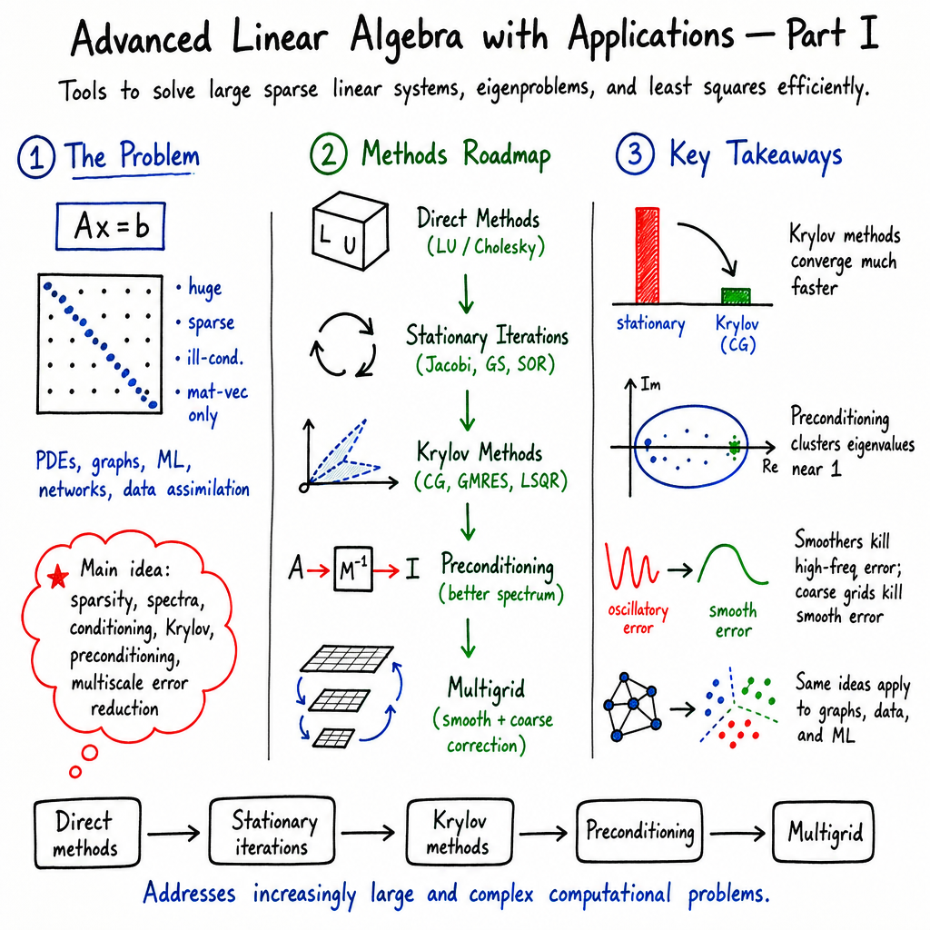
Abstract: These lecture notes form the first part of a master's-level course on advanced numerical linear algebra. Their aim is not only to present the classical algorithms, but to show why the subject has become considerably more central than it was a generation ago. Numerical linear algebra grew up alongside the numerical solution of partial differential equations, and for a long time that is where its large sparse systems came from. Ranking the nodes of a network, assimilating observations into a weather forecast, and fitting a model to a large noisy data set now lead to problems of the same kind: too large to factorise, structured, and accessible only through matrix-vector products. Strikingly few ideas are needed for all of them. Each chapter therefore develops a standard topic and then puts it to work outside its original setting. We treat norms, factorisations, conditioning and floating-point arithmetic; sparse matrices arising from finite differences, from graphs and from machine learning; stationary iterations and the smoothing property; the conjugate gradient and Lanczos methods, with spectral clustering and regularisation by early stopping; Arnoldi and GMRES, with PageRank and large least squares; and finally preconditioning, Schwarz domain decomposition and multigrid. We assume a first course in linear algebra. Every section closes with a summary of what should be retained and every chapter with exercises, several drawn from past examinations. Accompanying Python code reproduces the numerical illustrations.
Paper Prompts
Sign up for free to create and run prompts on this paper.
Top Community Prompts
Explain it Like I'm 14
1. Brief overview
This document is the first part of a set of lecture notes called Advanced Linear Algebra with Applications.
It explains how computers use linear algebra to solve large scientific and engineering problems. Linear algebra involves vectors, matrices, and systems of equations. These tools are used in:
- Weather forecasting
- Machine learning
- Data assimilation, such as combining weather observations with a forecast
- Graphs and networks
- Engineering simulations
- Solving differential equations
The main message is that many different real-world problems can be changed into a similar form:
Here, is a matrix, is the unknown answer, and contains known information.
The notes focus especially on how to solve these systems quickly, accurately, and with limited computer memory.
2. Main objectives and questions
The authors want students to understand several important questions:
- How can we measure the size of a vector, a matrix, or an error?
- Why are some mathematical problems very sensitive to small mistakes?
- How do computers represent numbers, and why do rounding errors happen?
- How can we solve using methods such as LU factorization or Cholesky factorization?
- Why do some methods work well for small systems but become too slow for huge systems?
- How can we solve very large systems by starting with a guess and improving it repeatedly?
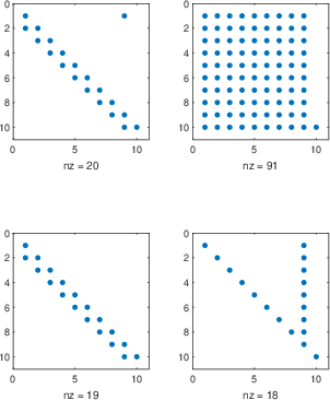
- Why are some matrices mostly filled with zeros, and how can this make calculations faster?
- How can differential equations be changed into matrix equations that a computer can solve?
In the part shown, the notes mainly develop the basic ideas needed for later chapters. These include norms, eigenvalues, conditioning, numerical errors, matrix factorizations, and iterative methods.
3. Research or teaching approach
This is not a research paper reporting one new experiment. It is a mathematical teaching text. The authors explain ideas, give definitions, prove important results, show examples, and provide exercises.
Measuring size with norms
A norm is a way of measuring the size or length of something.
For example, if a vector is
its usual Euclidean length is
This is like finding the distance from the center of a map to a point. Other norms measure size in different ways, such as adding all the absolute values or looking only at the largest value.
The notes explain that different norms may give different numbers, but in a finite-dimensional space they agree about whether something is becoming small or approaching zero.
Understanding eigenvalues and matrix decompositions
An eigenvector is a special direction that a matrix does not turn to a new direction. Instead, the matrix simply stretches or shrinks it:
The number is called the eigenvalue. An analogy is a rubber arrow being stretched by a machine without changing its direction.
The notes also introduce several ways to break a complicated matrix into simpler pieces:
- Eigendecomposition
- Schur decomposition
- Singular value decomposition, or SVD
These are useful because simpler pieces are often easier for a computer to study and calculate with.
Studying computer errors
Computers usually cannot store every real number exactly. Instead, they use floating-point arithmetic, which stores numbers with a limited number of digits.
This can cause:
- Rounding errors, when a number is shortened
- Truncation errors, when an infinite process is stopped early
- Cancellation errors, when two almost equal numbers are subtracted and many useful digits disappear
For example, subtracting two numbers such as $1.0000001$ and $1.0000000$ can be dangerous if the computer has already rounded them.
The notes use the condition number to describe how sensitive a problem is. A badly conditioned problem is like trying to balance a pencil on its tip: a very small disturbance can create a large change. Even a good computer algorithm may produce an unreliable answer for such a problem.
Comparing direct and iterative methods
The notes describe two major families of methods for solving matrix equations.
A direct method tries to solve the problem in a fixed sequence of steps. Gaussian elimination is an example. It changes a matrix into simpler triangular matrices using an LU factorization:
This is similar to taking a complicated set of instructions and breaking it into two simpler instruction lists.
For symmetric positive definite matrices, the authors describe Cholesky factorization:
Cholesky is faster and requires less storage than general LU factorization when it can be used.
An iterative method begins with a guess and repeatedly improves it. This is like trying to reach the correct location on a map by taking many small steps rather than calculating the entire route at once.
The notes discuss:
- Jacobi iteration
- Gauss–Seidel iteration
- Successive Over-Relaxation, or SOR
- Richardson’s method
These methods are especially useful when matrices are extremely large but contain mostly zeros. Such matrices are called sparse matrices.
A key test for whether an iterative method will converge is the size of its iteration matrix. In simplified terms, the repeated updates must gradually shrink the error rather than make it larger.
Changing differential equations into matrix problems
The second chapter begins explaining finite differences. A differential equation describes how a quantity changes continuously. Computers, however, usually work with a finite collection of points.
The authors replace derivatives with formulas involving nearby points. For example, the second derivative can be approximated by
This is like estimating the shape of a road by looking at the heights of three nearby locations.
The smaller the distance between points, the more accurate the approximation usually becomes. The notes explain this accuracy using the idea of truncation error.
4. Main findings and important ideas
Because this is a set of lecture notes, its “findings” are the mathematical conclusions and practical lessons it presents.
Large problems need special methods
Direct methods such as LU factorization can require roughly
operations. This means that the amount of work grows very quickly as the number of unknowns increases.
For a small system, this may be fine. For systems with millions or billions of unknowns, it is usually too expensive. Iterative methods are more suitable because each step can often use only the nonzero entries of the matrix.
Sparse matrices make large calculations possible
Many real-world problems have local connections:
- A point in a physical grid usually interacts only with nearby points.
- A person in a social network is connected to only some other people.
- A data feature may affect only certain parts of a model.
As a result, most matrix entries are zero. Storing and using only the nonzero entries saves time and memory.
Stability and conditioning both matter
The notes emphasize an important distinction:
- Conditioning describes how sensitive the problem itself is.
- Stability describes how well the algorithm handles errors.
A stable algorithm cannot completely fix a problem that is naturally very sensitive. However, an unstable algorithm can create large errors even when the original problem is easy.
Gaussian elimination with partial pivoting, which swaps rows to use safer pivot elements, is presented as an important way to improve stability.
Convergence depends on the right structure
Jacobi and Gauss–Seidel methods are guaranteed to converge for certain types of matrices, including many diagonally dominant matrices. Gauss–Seidel also converges for symmetric positive definite matrices.
SOR can speed up Gauss–Seidel when its relaxation parameter is chosen well. However, the parameter must be chosen carefully; for the important positive definite case, it must lie between $0$ and $2$.
Finite differences provide useful approximations
The finite-difference formulas show how a continuous differential equation can become a large system of algebraic equations. The standard three-point approximation for a second derivative has an error of order , meaning that making the grid spacing smaller generally makes the approximation much more accurate.
This explains where many sparse matrices in scientific computing come from.
5. Why the results matter
These ideas are important because modern computers often need to solve enormous mathematical problems.
For example, a weather model may involve billions of unknown values describing temperature, pressure, wind, and humidity. It would be impossible to treat such a problem as a small classroom system. Efficient sparse and iterative methods allow computers to obtain useful answers in a reasonable amount of time.
The same ideas can also help:
- Train machine-learning models
- Rank websites or network nodes
- Improve weather forecasts using new observations
- Simulate bridges, airplanes, and buildings
- Model heat, fluid flow, and pollution
- Solve optimization and data-analysis problems
The notes also warn that getting an answer is not enough. We must ask whether the answer is accurate and whether small computer errors could have changed it significantly.
Simple conclusion
The document teaches a toolkit for solving large systems of equations on computers. Its central idea is that many different problems—from weather prediction to machine learning—can be handled using the same mathematical concepts.
The most important lessons are:
- Matrices can represent many kinds of real-world relationships.
- Sparse matrices save computer time and memory.
- Some problems are naturally sensitive to small errors.
- Stable algorithms help control computer mistakes.
- Iterative methods are often better than direct methods for huge systems.
- Finite differences turn difficult differential equations into matrix equations.
The potential impact of this work is educational and practical. By learning these ideas, students gain the foundation needed to design and understand fast computer methods used in science, engineering, artificial intelligence, and data analysis.
Knowledge Gaps
Knowledge gaps, limitations, and open questions
- The manuscript is incomplete: the supplied text ends during the proof of the three-point finite-difference truncation result, so the stated coverage of 2D PDEs, graph Laplacians, machine learning, data assimilation, sparse storage, reordering, Krylov methods, preconditioning, domain decomposition, and multigrid is not actually developed.
- The notes do not establish how the presented methods perform on realistic large-scale systems, despite motivating applications involving up to unknowns; systematic benchmarks varying problem size, sparsity pattern, hardware, and memory constraints are absent.
- The relationship between discretization error, algebraic solver error, floating-point error, and total application-level error is not quantified; future work should provide end-to-end error budgets for representative PDE problems.
- Boundary conditions, variable coefficients, nonuniform grids, irregular domains, and nonsmooth solutions are not analyzed, leaving the stated finite-difference accuracy results unresolved for common practical PDE settings.
- Stability and convergence are treated primarily for simple stationary iterations, while stability of the full discretize–solve pipeline is not examined, particularly for nonnormal, nonsymmetric, indefinite, or singular matrices.
- The discussion of convergence based on does not explain how the spectral radius or relevant norm can be estimated inexpensively in practice; practical stopping and parameter-selection procedures therefore remain unspecified.
- The claimed near-optimality of SOR parameters is not evaluated when the Jacobi eigenvalues are complex, when is unavailable, or when the matrix is nonsymmetric or poorly scaled.
- No analysis is provided of how matrix scaling, diagonal equilibration, ordering, or variable rescaling affect conditioning and the convergence of Jacobi, Gauss–Seidel, SOR, and Richardson methods.
- The notes state that Gauss–Seidel is backward stable for SPD matrices and that GEPP is backward stable, but do not provide precise assumptions, norm-dependent constants, growth-factor bounds, or finite-precision error estimates needed to assess these claims quantitatively.
- The floating-point model is presented incompletely and with no treatment of subnormal numbers, overflow, underflow, fused multiply–add operations, reproducibility, or deviations across CPU/GPU architectures.
- Reduced- and mixed-precision methods are mentioned but not analyzed experimentally or theoretically; the effects of precision placement, iterative refinement, preconditioner precision, and loss of attainable accuracy remain open.
- The treatment of condition numbers focuses mainly on perturbations in and does not fully characterize perturbations in , componentwise error, normwise versus componentwise backward error, or the distinction between residual size and solution accuracy.
- The statement that a small residual or residual-based backward error indicates solution quality is not accompanied by conditions under which this inference is reliable, especially for ill-conditioned or badly scaled systems.
- Sparse direct-solver complexity is summarized using asymptotic expressions, but fill-in and computational cost are not related to graph structure, nested dissection, minimum degree ordering, separator quality, or three-dimensional PDE discretizations.
- No comparative study determines when sparse direct methods become preferable to iterative methods, taking into account setup costs, multiple right-hand sides, parallelism, robustness, memory, and preconditioner construction.
- The notes do not investigate convergence deterioration with mesh refinement, although this is central for elliptic PDEs; the dependence of iteration counts on , dimension, coefficient contrast, and anisotropy is left unexplored.
- The role of stationary iterations as multigrid smoothers is asserted but not demonstrated; smoothing factors, high- versus low-frequency error reduction, and suitable choices for anisotropic or heterogeneous problems are not derived.
- Nonnormality and transient growth are omitted, so the presentation does not explain why eigenvalues alone can be insufficient to predict finite-iteration behavior for nonsymmetric problems.
- The treatment does not address breakdown, stagnation, loss of orthogonality, or residual-gap phenomena in finite-precision iterative methods.
- The practical design and effectiveness of preconditioners are not yet covered in the supplied text, including incomplete factorizations, algebraic multigrid, domain decomposition, block preconditioners, and methods for indefinite or saddle-point systems.
- No criteria are given for choosing between Jacobi, Gauss–Seidel, SOR, Richardson, direct solvers, and Krylov methods for specific matrix classes or application constraints.
- The claimed transferability of methods between PDE matrices, graph Laplacians, machine-learning matrices, and data-assimilation systems is not validated; these applications differ substantially in symmetry, definiteness, conditioning, sparsity, and data noise.
- The machine-learning discussion does not examine rank deficiency, overparameterization, stochastic optimization, implicit regularization, or the numerical consequences of solving normal equations versus using QR or SVD methods.
- The data-assimilation discussion does not quantify the effects of localization, covariance approximation, observation density, model error, or changing correlation length scales on matrix conditioning and solver performance.
- The notes provide no reproducible experimental results from the referenced Python repository, including software versions, hardware, parameter settings, convergence tolerances, or comparisons with established libraries.
- The pedagogical exercises are not accompanied by solutions, numerical validation, or error analyses, making it unclear whether they adequately test the theoretical and practical claims.
- Several displayed formulas and LaTeX definitions in the supplied manuscript contain apparent syntax or transcription errors, so the mathematical statements and executable examples require systematic verification before the notes can serve as a reliable reference.
- The manuscript does not discuss the limits of the presented finite-dimensional theory for very large-scale, distributed-memory, randomized, streaming, or out-of-core settings.
- Open questions remain concerning robust solver behavior under time-varying matrices, repeated solves, multiple right-hand sides, noisy data, dynamically changing sparsity patterns, and heterogeneous parallel hardware.
Practical Applications
Immediate Applications
- Scientific computing and engineering simulation — scalable sparse linear-system solvers. Implement finite-difference discretizations of 1D/2D Poisson-type PDEs and solve the resulting sparse systems with Jacobi, Gauss–Seidel, SOR, LU, or Cholesky methods. This is directly applicable to heat transfer, electrostatics, diffusion, structural mechanics, and fluid-flow subproblems. Sparse storage formats such as CSR/CSC can reduce memory use, while iterative updates cost approximately per step. Dependencies: The discretized matrix must have appropriate structure; convergence of stationary methods depends on conditions such as strict diagonal dominance, symmetric positive definiteness (SPD), or . Grid refinement can make systems increasingly ill-conditioned, requiring preconditioning.
- Finite-difference PDE software and educational tools. The paper’s formulas for forward, backward, central, and second-derivative differences can be integrated into Python/SciPy teaching notebooks or lightweight simulation packages. Users can vary grid spacing , boundary conditions, and solver tolerances to observe truncation error, convergence, and roundoff effects. Dependencies: The underlying solution should be sufficiently smooth for the stated truncation orders; boundary treatment and stability analysis must be added for time-dependent or nonlinear PDEs.
- Engineering and scientific solver selection workflows.
- use Cholesky for well-scaled SPD systems;
- use LU with partial pivoting for general moderate-sized systems;
- use iterative methods for very large sparse systems;
- estimate conditioning and monitor residuals before trusting the computed solution.
- This can be embedded in numerical libraries, simulation pipelines, and quality-control reports.
- Dependencies: Matrix classification must be reliable, and a small residual alone cannot guarantee a small forward error when is large.
- Numerical reliability and verification in safety-critical software. Condition numbers, forward error, backward error, residuals, machine precision, and overflow checks can be incorporated into validation workflows for aerospace, automotive, energy, medical imaging, and industrial control software. Partial pivoting should be enabled in general LU implementations, and precision changes should be tested explicitly. Dependencies: Error bounds are estimates rather than guarantees of application-level correctness; scaling, model error, discretization error, and implementation defects must also be evaluated.
- Data assimilation and weather forecasting — sparse correlation systems. Localized or compactly supported observation-correlation matrices, such as SOAR-type matrices mentioned in the paper, can be stored and solved using sparse iterative methods. This supports workflows that combine model forecasts with sensor or satellite observations. Dependencies: Correlation localization must preserve a suitable matrix structure, often SPD; convergence and accuracy depend on observation geometry, correlation length scales, conditioning, and solver tolerances.
- Machine learning and large-scale least-squares computation. The same sparse-matrix principles apply to normal equations, Hessian approximations, regularized least squares, and feature matrices. SVD-based diagnostics can identify rank deficiency, while conditioning analysis can guide regularization through transformations such as . Dependencies: Forming normal equations can square the condition number, so QR, SVD, or appropriately preconditioned iterative methods may be preferable. Sparsity depends on the feature representation and may be lost during matrix operations.
- Graph analytics and network computation. Graph Laplacians can be constructed from edge lists and processed using the same sparse iterative techniques as PDE matrices. Immediate uses include network smoothing, diffusion processes, connectivity diagnostics, ranking-related linear systems, and spectral graph preprocessing. Dependencies: The graph must be represented accurately, and the relevant Laplacian may be singular because of disconnected components or constant-vector nullspaces. Solver choice must account for this structure.
- Software libraries and reproducible computational workflows. The accompanying Python examples can serve as templates for reproducible experiments involving matrix norms, condition numbers, LU/Cholesky factorization, stationary iterations, sparse storage, and convergence histories. These components could be packaged as diagnostic utilities for research code. Dependencies: The repository and numerical examples must be maintained, tested across hardware and precision levels, and corrected for implementation or notation errors in the supplied manuscript.
- Daily-life and general computing — numerical robustness awareness. The paper’s principles can inform practical choices such as avoiding subtraction of nearly equal quantities, checking for overflow in type conversions, using stable summation orders, and validating results with residuals or independent calculations. These ideas are relevant to spreadsheets, financial calculators, sensor-processing scripts, and personal data-analysis code. Dependencies: Users need access to diagnostic information such as data ranges, precision, and condition estimates; simple checks cannot replace domain-specific validation.
Long-Term Applications
- Production-scale PDE solvers using multigrid and domain decomposition. The stationary methods described as smoothers can form components of multigrid solvers, while domain decomposition can distribute large engineering or geophysical simulations across CPU/GPU clusters. Such systems could support higher-resolution climate, seismic, electromagnetic, and structural simulations. Dependencies: The excerpt is foundational and does not provide a complete multigrid or domain-decomposition implementation. Scalability depends on parallel communication, robust coarse-grid construction, boundary conditions, heterogeneous coefficients, and effective smoothers.
- GPU- and accelerator-oriented mixed-precision solvers. Reduced precision can accelerate sparse matrix–vector products and PDE model evaluations, while higher precision can be reserved for residual correction, factorization safeguards, or convergence verification. This could reduce energy consumption and runtime in machine learning, data assimilation, and scientific computing. Dependencies: Mixed precision requires error analysis, reliable stopping criteria, hardware support, and safeguards for ill-conditioned systems. Lower precision may cause stagnation, loss of positive definiteness, overflow, or misleading residuals.
- Large-scale weather and climate data assimilation. Combining sparse correlation models, iterative solvers, domain decomposition, and mixed precision could enable faster assimilation of dense satellite and sensor data into forecasts. Potential products include operational assimilation engines with adaptive solver and precision selection. Dependencies: The full workflow requires nonlinear model integration, observation-error modeling, parallel implementations, uncertainty quantification, and strict operational reliability. The paper addresses the linear-algebra foundation rather than the complete forecasting system.
- Spectral graph machine learning and network intelligence. Eigenvalue and SVD computations, graph Laplacians, and sparse Krylov methods could support future tools for graph embeddings, community detection, recommendation, anomaly detection, transportation analysis, and communication-network monitoring. Dependencies: Large-scale spectral methods require efficient eigensolvers, scalable preconditioners, dynamic-graph support, and validation that the extracted spectral features are meaningful for the target domain.
- Large-scale optimization and training of machine-learning models. Krylov methods, conditioning diagnostics, regularization, and Hessian-vector products could be developed into second-order or hybrid optimization tools that avoid explicitly forming dense Hessians. Early stopping may also act as an implicit regularizer in inverse or statistical problems. Dependencies: The excerpt only establishes the relevant numerical concepts; practical deployment requires algorithms for nonconvex, stochastic, distributed, and dynamically changing objectives, along with convergence and generalization studies.
- Digital twins and real-time engineering control. Fast sparse PDE solvers and reduced-precision iterative methods could become components of digital twins for aircraft, factories, power systems, buildings, and robotic platforms. These systems could update simulated states in real time from sensor observations. Dependencies: Real-time use requires strict latency guarantees, robust handling of changing meshes and parameters, model-reduction techniques, uncertainty quantification, and fault-tolerant solver switching.
- Policy and regulatory standards for numerical reliability. The paper’s emphasis on conditioning, backward stability, pivoting, precision, and residual monitoring could inform standards requiring numerical-risk assessments for safety-critical computational models. Possible artifacts include solver audit logs, precision declarations, conditioning thresholds, and reproducibility requirements. Dependencies: Numerical diagnostics must be translated into sector-specific risk criteria. Conditioning alone does not capture modeling errors, biased data, software defects, or inappropriate physical assumptions.
- Automated adaptive solver-selection systems. Future scientific-computing platforms could inspect matrix sparsity, symmetry, definiteness, estimated spectrum, condition number, and hardware availability, then automatically select among Cholesky, LU, Jacobi, Gauss–Seidel, SOR, Krylov, multigrid, and mixed-precision variants. Dependencies: Reliable matrix classification and spectral estimation can themselves be computationally costly. Such systems require extensive benchmarking across matrix families and safeguards against incorrect convergence assumptions.
- High-assurance numerical computing for safety-critical applications. Aerospace guidance, medical imaging, nuclear-energy simulation, autonomous robotics, and financial risk systems could combine backward-error analysis, interval or probabilistic error bounds, redundant computation, and precision-aware algorithms. Dependencies: The paper provides core numerical concepts but not formal verification, interval arithmetic, uncertainty propagation, or certification procedures. Regulatory acceptance would require application-specific testing and demonstrable worst-case guarantees.
Glossary
- Arnoldi method: An iterative algorithm that constructs an orthonormal basis for a Krylov subspace and produces an upper Hessenberg matrix. “Arnoldi and GMRES, with PageRank and large least squares”
- Backward error: The smallest perturbation to the input data that makes a computed solution exact. “backward error ”
- Backward stability: A property of an algorithm that guarantees its computed result is the exact solution to a nearby problem. “Gaussian elimination with partial pivoting (GEPP) is backward stable”
- Banded matrix: A matrix whose nonzero entries are concentrated near its main diagonal. “For sparse banded matrices with half-bandwidth ”
- Bandwidth: The maximum distance of a nonzero matrix entry from the main diagonal. “explain how bandwidth, profile, and reordering affect fill-in and solver cost”
- Catastrophic cancellation: Severe loss of significant digits caused by subtracting nearly equal numbers. “This is an example of catastrophic cancellation, where most significant digits cancel out.”
- Cholesky factorization: A factorization of a symmetric positive-definite matrix into a lower-triangular matrix and its transpose. “If is SPD, then ”
- Condition number: A measure of how sensitively a problem’s solution responds to perturbations in its input. “For a nonsingular , ”
- Conjugate gradient: An iterative method for solving symmetric positive-definite linear systems using mutually conjugate search directions. “conjugate gradient and Lanczos, with spectral clustering and regularisation by early stopping”
- Consistency: The property that a discretized differential operator approaches the corresponding continuous operator as the discretization is refined. “A finite difference operator is consistent with a differential operator ”
- Domain decomposition: A numerical technique that divides a computational domain into smaller subdomains to enable efficient solution, often in parallel. “and finally preconditioning, domain decomposition and multigrid.”
- Eigendecomposition: A representation of a diagonalizable matrix in terms of its eigenvectors and eigenvalues. “it admits an eigendecomposition”
- Fill-in: New nonzero entries created in matrix factors during elimination of a sparse matrix. “Fill-in during elimination destroys sparsity”
- Finite difference method: A discretization technique that approximates derivatives using values of a function at neighboring grid points. “Three of the most common approaches include the finite element method, finite volume method, and finite difference method.”
- Floating-point model: A mathematical model describing how real numbers and arithmetic operations are represented approximately on a computer. “A real number is represented as:”
- Frobenius norm: The square root of the sum of the squared absolute values of all matrix entries. “The most important exception is the Frobenius norm”
- GMRES: An iterative Krylov-subspace method for solving nonsymmetric linear systems by minimizing the residual over expanding subspaces. “Arnoldi and GMRES, with PageRank and large least squares”
- Graph Laplacian: A matrix representing the connectivity structure of a graph, commonly defined as the degree matrix minus the adjacency matrix. “Define the graph Laplacian ”
- Half-bandwidth: The maximum number of diagonal positions separating a nonzero entry from the main diagonal on one side. “with half-bandwidth , the costs are ”
- Ill-conditioned: Describing a problem for which small input perturbations can cause large changes in the output. “The Hilbert matrix is symmetric positive definite, but extremely ill-conditioned.”
- Induced norm: A matrix norm measuring the maximum factor by which a matrix can enlarge vectors under a specified vector norm. “For a matrix the {induced norm (operator norm)} is defined by”
- Krylov subspace: A subspace generated by successive applications of a matrix to a vector, typically . “Sparsity, the spectrum, Krylov subspaces and preconditioning recur throughout”
- Lanczos method: An iterative procedure for generating an orthogonal basis of a Krylov subspace for symmetric matrices, producing a tridiagonal projection. “conjugate gradient and Lanczos, with spectral clustering”
- Least squares: A method for finding parameters that minimize the squared residual between observed and modeled data. “Arnoldi and GMRES, with PageRank and large least squares”
- Machine epsilon: The smallest positive floating-point number that changes the stored value of $1$ when added to it. “The machine epsilon $\varepsilon_{\text{mach}$ is the smallest number such that”
- Matrix splitting: The decomposition of a matrix into two matrices, commonly written , to define an iterative method. “Let with invertible.”
- Multigrid: A class of iterative methods that accelerates the solution of discretized differential equations by combining computations on multiple grid resolutions. “Jacobi, GS, and SOR remain indispensable as smoothers in multigrid”
- Neumann series: An infinite matrix series that expresses an inverse as when the series converges. “Equivalently, the Neumann series converges”
- Normal equations: Linear equations obtained by setting the gradient of a least-squares objective to zero, typically in the form . “the normal equations of a machine learning model”
- Partial pivoting: A Gaussian-elimination strategy that swaps rows to use a suitably large pivot element. “During elimination, rows are swapped to ensure that pivot elements are large in magnitude.”
- Preconditioner: An operator used to transform a linear system into an equivalent one that is easier for an iterative solver to solve. “This motivates the use of iterative solvers and preconditioners.”
- Schur decomposition: A factorization of a square matrix into a unitary matrix, an upper-triangular matrix, and the unitary conjugate transpose. “Every admits a Schur decomposition”
- Singular value decomposition (SVD): A factorization expressing a matrix as two unitary matrices surrounding a diagonal matrix of singular values. “Every (or ) admits a singular value decomposition (SVD)”
- Spectral clustering: A graph-partitioning technique that uses eigenvectors of a graph-related matrix to identify clusters. “conjugate gradient and Lanczos, with spectral clustering”
- Spectral radius: The largest absolute value of a matrix’s eigenvalues. “The spectral radius is .”
- Stationary iteration: An iterative method whose update has a fixed matrix form, such as . “Define the stationary iteration”
- Stencil: A fixed local pattern of neighboring grid points used to approximate a differential operator. “whose nonzero pattern is dictated by local structure - a stencil”
- Subordinate norm: A matrix norm induced by a vector norm and satisfying . “there exists a (subordinate) norm ”
- Successive over-relaxation (SOR): An iterative method that accelerates Gauss–Seidel by weighting updates with a relaxation parameter. “Successive Over-Relaxation (SOR)”
- Truncation error: The local error introduced when an infinite or continuous mathematical operation is approximated by a finite or discrete one. “The term is the local truncation error”
- Unitary matrix: A complex matrix whose conjugate transpose is its inverse. “with unitary and ”
- Weighted infinity norm: A vector norm that scales each component by a positive weight before taking the maximum. “An idea would be to use a weighted -norm ”