A cornucopia of null results: A statistical analysis of fireballs reported to the American Meteor Society
Abstract: In March 2026, the American Meteor Society announced that a "surge" of large fireballs had been reported to their website in the first quarter of the year, and that these fireballs had certain characteristics (radiant clustering and reports of delayed sound). We find this data set to be an excellent use case for Poisson regression, which, in our opinion, is underutilized in meteor astronomy. This report serves as a brief primer on Poisson regression and related statistical techniques as well as an analysis of AMS fireball counts. We find that the number of events reported in early 2026 is in line with the overall pattern of activity. We also find little evidence of the "February fireballs" phenomenon.
Paper Prompts
Sign up for free to create and run prompts on this paper using GPT-5.
Top Community Prompts
Explain it Like I'm 14
A simple guide to “A cornucopia of null results: A statistical analysis of fireballs reported to the American Meteor Society”
What this paper is about (big picture)
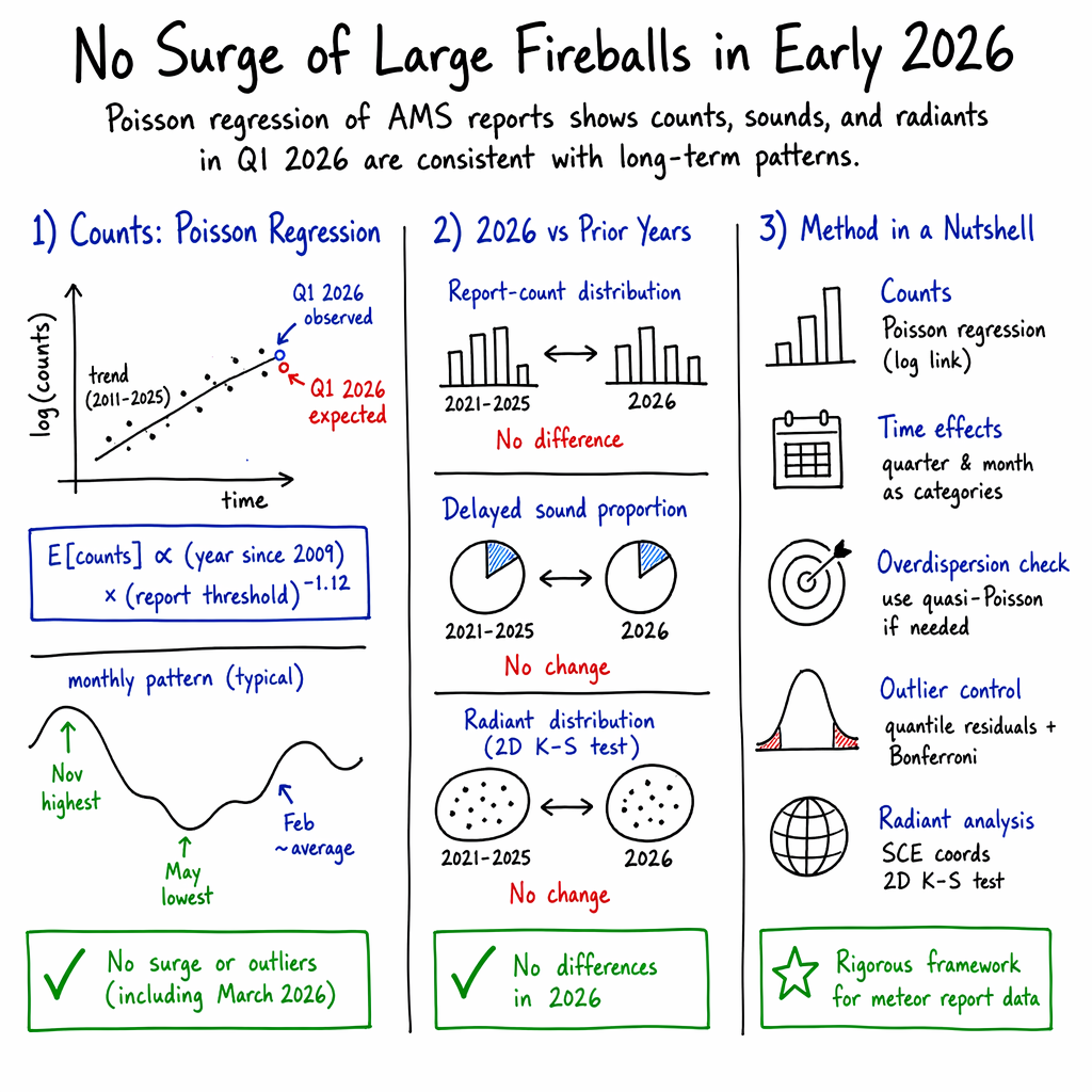
This paper asks a straightforward question: Were there really more big meteors (“fireballs”) than usual in early 2026, like the American Meteor Society (AMS) suggested? The authors check the AMS’s claims using careful statistics. Their main message: once you account for normal growth in reports and seasonal patterns, early 2026 looked normal. In short, no clear surge.
1) Main topic or purpose
The paper investigates whether there was an unusual spike in reported fireballs in the first quarter of 2026 and examines several related claims (like special sky patterns and reports of delayed sounds). It also teaches a useful statistical tool—Poisson regression—showing how to analyze counts of events properly.
2) Key objectives in simple terms
The authors set out to:
- Check if the number of reported fireballs in early 2026 was unusually high.
- See if any increase was strongest for the biggest events (those with lots of eyewitness reports).
- Test whether March 2026 stood out compared to other months.
- Check if more fireballs than usual were reported to make delayed sounds.
- See if fireballs came from unusually clustered directions in the sky.
- Show how to use better coordinates for mapping meteor directions (Sun-centered ecliptic) and how to use proper “fair-play” statistics when doing lots of tests at once.
Two AMS claims couldn’t be tested because the necessary data weren’t available or the definition wasn’t clear:
- Whether there were more long-duration fireballs.
- Whether there were more “major” fireballs (the term wasn’t clearly defined).
3) How they did it (methods made simple)
Think of counting fireballs like counting raindrops in different buckets over time. The team used tools that are designed for counting events:
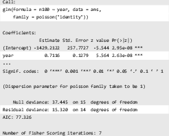
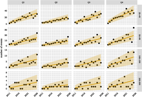
- Poisson regression: This is a model that helps predict counts (like number of fireballs) from things like time (year) and “size” (how many reports an event got). It’s great for situations where events are rare and can be 0, 1, 2, and so on—like raindrops hitting a bucket. It also assumes events happen independently.
- Generalized Linear Models (GLMs): Like a more flexible version of straight-line fits; they let you connect predictors to the average count in a smart way (for counts, you often use a log link).
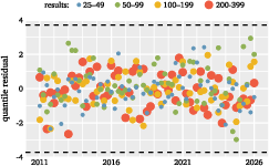
- Residuals: After fitting a model, you look at what’s left over (the “residuals”) to see if the model missed anything big. If residuals look random, your model is probably fine.
- Multiple comparisons (Bonferroni correction): If you test many different things, you’re more likely to find a “lucky” false hit. Bonferroni is like tightening the rules when you run lots of tests, so you don’t fool yourself.
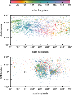
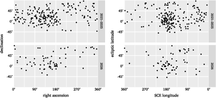
- Sun-centered ecliptic (SCE) coordinates: A better map for meteor directions. Imagine rotating your map so important features line up; here, centering on the Sun and Earth’s motion makes meteor patterns easier to see and compare.
- Fisher’s exact test: A careful way to compare proportions (like the fraction of events with delayed sound) when sample sizes are small.
- Two-dimensional K–S test: A way to compare two distributions in 2D (like sky directions) to see if one year looks different from others.
Data sources and choices:
- The team analyzed AMS website data from 2011 to early 2026 (the reporting system improved around 2010).
- They grouped events by the number of reports (25–49, 50–99, 100–199, 200–399, etc.) so each group contains independent counts.
- They looked by year, quarter, and month.
- They used SCE coordinates to check whether fireball directions were unusually clustered.
- They found the AMS API had inconsistencies with the website (different report counts and even very different directions), so they stuck with website data to match the AMS’s public analysis.
Everyday analogy:
- Imagine you’re checking if a school had “way more” tardies in one term. If the school has grown steadily for years, seeing more tardies this year might just be normal growth. You’d also check if certain months are naturally busier (like winter) before calling anything unusual. That’s what the authors did—but with meteors.
4) Main findings and why they matter
Here’s what they found, put simply:
- No unusual surge in early 2026:
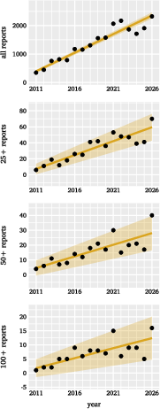
- The number of reported fireballs has been growing steadily over the years (likely because more people report them, or better tools, or both).
- Early 2026 fits that steady trend. It didn’t stick out as a spike once you account for the ongoing growth.
- Bigger events weren’t unusually common:
- If 2026 were special, you might expect especially strong increases among the biggest fireballs (those with lots of reports). That didn’t happen.
- March 2026 was normal for its time of year:
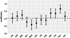
- They modeled month-by-month patterns and found a seasonal rhythm (November tends to be higher, May lower).
- February was average—no special “February fireball” effect showed up in these data.
- March 2026 didn’t look unusual when you consider the overall month patterns plus the steady year-to-year growth.
- “Delayed sound” reports didn’t spike:
- The fraction of events with delayed sound (booms heard after the flash) wasn’t significantly different in early 2026 compared to earlier years.
- Sky directions weren’t weird:
- The directions the meteors came from in 2026 looked similar to previous years when checked properly (including with SCE coordinates).
- The data for directions had some big uncertainties—sometimes very big—so any strong direction-based claim needs caution.
- Important caution on low-report events:
- Very low-report counts (like single-report events) were “noisier” than expected (overdispersed). That might be due to weather, visibility, or misreports. The team downplayed those and focused on better-quality bins (25+ reports).
Why this matters:
- It’s easy to be misled by raw counts, especially when the reporting community grows.
- Using the right tools (like Poisson regression) and fair rules (like Bonferroni correction) helps avoid false alarms.
- Choosing the right sky map (SCE) makes patterns clearer and comparisons fairer.
5) What this means going forward (implications)
- For the public and media: The sky didn’t suddenly get more “fireball-y” in early 2026—at least not in a way that stands out from normal growth and seasonal patterns. Headlines about a “surge” were likely due to not accounting for those trends.
- For researchers and citizen scientists:
- Poisson regression is a powerful, underused tool for meteor counts. It handles zeros and small numbers well.
- Always check residuals and adjust for multiple tests to avoid fooling yourself.
- Use SCE coordinates for radiant clustering studies.
- Be cautious with low-report or uncertain data, and be transparent about definitions (like what counts as a “major” fireball).
- For future work:
- Better, more consistent data (including event durations and well-defined categories) will help test myths like “February fireballs” more reliably.
- Sharing clear methods and open code, as the authors did, encourages trustworthy, repeatable science.
In short, the authors found “null results”—they didn’t confirm a special surge—but that’s valuable. It helps set the record straight and shows how to analyze meteor reports in a fair, careful way.
Knowledge Gaps
Below is a concise list of concrete knowledge gaps, limitations, and open questions that remain unresolved in the paper and that future work could address:
- Resolve and document discrepancies between AMS website and API datasets (report counts and radiants), establish an authoritative, versioned data export, and quantify their impact on results.
- Audit the AMS data-processing pipeline to identify why ~1/3 of compared events show >90° radiant discrepancies; publish reproducible logs of recalculations, merging, and event updates.
- Determine whether listed radiants are apparent or geocentric, compute per-event radiant uncertainties, and propagate them through radiant-distribution tests and clustering analyses.
- Use uncertainty-aware, exposure-aware two-sample tests on the sphere (e.g., permutation tests with spherical kernels, energy distance/MMD) rather than 2D K–S, and explicitly model non-uniform sky visibility and daytime masking.
- Extend radiant-clustering analyses beyond Q1 to all quarters (and years) to test seasonal robustness of null results.
- Collect and incorporate exposure covariates (observer counts, geographic density, site traffic/app usage, outreach/media spikes, cloud cover, moon phase, hours of darkness) as offsets in GLMs to separate reporting effort from true event rates.
- Model overdispersion and potential false positives in low-report-count bins using negative binomial or zero-inflated/mixture models; estimate the fraction and characteristics of non-meteor reports.
- Test and correct the independence assumption by detecting near-simultaneous or duplicate events (time/radiant/trajectory proximity), and if necessary use clustered/robust standard errors or self-exciting point-process models.
- Compare alternative temporal trends (linear, log-linear, piecewise, and logistic growth) and test for structural breaks tied to platform changes (2016–2018), UI updates, or outreach campaigns.
- Calibrate or develop correction factors to bring pre-2011 data into a unified analysis, enabling longer-term trend assessments with quantified uncertainty.
- Quantify and correct for report-accumulation lag (time to stabilize event counts); ensure comparisons use consistent “as-of” cut dates across years.
- Cross-validate AMS-derived trends against independent instrumental datasets (e.g., NASA All Sky Fireball Network, GMN, CNEOS bolides, infrasound) to disentangle reporting growth from true meteoroid flux changes.
- Define objective criteria for “major” fireballs (e.g., peak magnitude, radiated energy, end height, fragmentation metrics) and re-test claim #4 within that standardized framework.
- Acquire, validate, and standardize duration data (claim #6): assess inter-rater reliability, UI effects on duration entry, and model duration as a function of geometry and energy proxies before testing 2026 anomalies.
- Re-examine delayed-sound claims with multivariable logistic (or hierarchical) models that include distance-to-trajectory, energy proxies (e.g., report count), time-of-day, atmospheric conditions, and regional effects to control for reporting bias.
- Quantify regional coverage biases (AMS is North America–centric) and fit spatiotemporal models (e.g., hierarchical Poisson/negative binomial with spatial random effects) to separate geographic heterogeneity from temporal changes.
- Investigate whether the power-law relation with report threshold (β_rep ≈ −1.12) varies by year, month, region, or shower activity; formally test interactions and nonstationarity.
- Explore whether month-specific patterns are better explained by known sporadic sources and shower calendars in SCE coordinates via forward simulations that include visibility and exposure masks.
- Evaluate sensitivity of conclusions to model-family choices (Poisson vs quasi-Poisson vs negative binomial) and link functions; report dispersion parameters and compare fits via information criteria and residual diagnostics.
- Provide predictive uncertainty that jointly accounts for parameter uncertainty and overdispersion; perform (Bayesian) posterior predictive checks or frequentist simulation-based calibration.
- Develop transparent deduplication/merging rules for events and publish open algorithms/IDs linking raw reports to events and events to revised solutions to improve reproducibility.
- Reassess the “February fireballs” lore using exposure-corrected metrics and physically meaningful event attributes (e.g., deep-penetrating/low end-height, high mass) rather than raw report counts.
- Assess statistical power to detect true surges at different thresholds and months; complement Bonferroni with FDR-based procedures, and report the smallest detectable effect sizes under realistic exposure.
- Document and freeze the exact AMS data snapshot used in analyses (with checksums) and provide end-to-end, executable workflows to ensure full reproducibility of results.
Practical Applications
Overview
Below are practical, real‑world applications grounded in the paper’s findings, methods, and innovations (Poisson regression workflow for count data, quantile residuals and multiple‑comparison control, Sun‑Centered Ecliptic coordinates for radiant analysis, and empirical trends in AMS reports). Applications are grouped by time‑to‑deployment and linked to sectors. Each item notes potential tools/products/workflows and key assumptions/dependencies that affect feasibility.
Immediate Applications
These can be deployed now with existing data and off‑the‑shelf tools (R statsmodels/GLM, Python, basic data engineering).
- Bold anomaly detection and reporting hygiene for meteor networks
- Sectors: software, research infrastructure, media/policy comms
- What: Implement a Poisson GLM dashboard for event counts with quantile residuals, overdispersion checks, and Bonferroni‑adjusted outlier flags to decide when a “surge” is statistically credible.
- Tools/workflows: R or Python GLM (Poisson/quasi‑Poisson), residual diagnostics, automated monthly/quarterly reports; alerting when residuals exceed adjusted thresholds.
- Assumptions/dependencies: Event independence; stable data pipeline; transparent α thresholds; acknowledgement of seasonal/monthly baselines.
- Data quality triage for low‑report events
- Sectors: software, operations, research
- What: Treat events with <25 reports as higher‑variance/noisier; route them through stricter validation (e.g., cross‑checks with weather, aircraft/satellite databases) given the paper’s documented overdispersion.
- Tools/workflows: Rule‑based filters; confidence scores by report band (25–49, 50–99, …).
- Assumptions/dependencies: Overdispersion reflects reporting bias/misidentification rather than physics; access to ancillary datasets (weather, traffic, flight paths).
- Operational forecasting for moderation and staffing
- Sectors: software, operations
- What: Use the fitted scaling laws to forecast expected report volumes by month and report threshold for resource planning.
- Tools/workflows: Use scaling and monthly coefficients to estimate weekly/monthly ticket loads; capacity planning dashboards.
- Assumptions/dependencies: Continued linear growth trend; platform usage growth roughly monotonic and not shock‑driven.
- Communications guidelines to reduce false “surge” narratives
- Sectors: policy, media relations, public outreach
- What: Codify a release checklist that requires (a) model‑based expected counts, (b) residual/outlier tests with multiple‑comparison corrections, and (c) uncertainty language before public claims.
- Tools/workflows: Press templates with p‑values after Bonferroni adjustment; plots with prediction intervals; standardized definitions (e.g., what constitutes “major”).
- Assumptions/dependencies: Organizational buy‑in; media partners willing to use standardized language.
- SCE‑based radiant analysis in observatories and education
- Sectors: astronomy/academia, education, software
- What: Adopt Sun‑Centered Ecliptic (SCE) coordinates in routine plots to make shower structure and sporadic sources clearer; reduce confounds from nodal precession and time‑of‑year effects.
- Tools/workflows: Scripts converting equatorial to SCE; side‑by‑side SCE/equatorial dashboards; classroom labs illustrating radiant clustering.
- Assumptions/dependencies: Accurate event times; clarity on apparent vs geocentric radiants.
- Two‑sample distribution checks for claimed radiant clustering
- Sectors: research, software
- What: Standardize on 2D K‑S tests (or alternatives) in SCE space for year‑over‑year distribution comparisons instead of ad‑hoc region picking.
- Tools/workflows: K‑S test modules; reproducible notebooks and cut‑lines that avoid slicing through dense regions.
- Assumptions/dependencies: Robust handling of spherical wrap‑around; sample sizes sufficient for nonparametric tests.
- API/data QA and provenance auditing
- Sectors: software/data governance, research infrastructure
- What: Automated linting to detect inconsistencies between API and website tables (report totals, radiants); provenance tags when radiants are revised; flags for >90° discrepancies.
- Tools/workflows: Nightly diff jobs; data dictionaries that specify apparent vs geocentric, uncertainty reporting, and recomputation triggers.
- Assumptions/dependencies: Access to both API and website data; versioning of derived products.
- Rapid proportion tests for “delayed sound” reports
- Sectors: public safety, aviation, emergency management
- What: On‑the‑fly Fisher’s exact tests by report band to decide whether current “boom/bang” call volume is unusual; triage for 911/aviation noise events.
- Tools/workflows: Small‑n safe stats (Fisher’s test) embedded in dispatch dashboards; thresholds for escalation.
- Assumptions/dependencies: Timely ingestion of reports; consistent tagging of “sound” field.
- GLM training modules for meteor astronomy and citizen‑science analytics
- Sectors: academia, research methods, data science upskilling
- What: Course labs that mirror the paper’s Poisson regression, quantile residuals, and multiple‑comparison workflows; template R/Python notebooks.
- Tools/workflows: Open lesson plans; version‑controlled repositories; CI to verify analyses.
- Assumptions/dependencies: Institutional adoption; access to open data.
Long‑Term Applications
These require additional research, standardization, covariates, or system integration before reliable deployment.
- Bias‑aware flux estimation via hierarchical/Bayesian GLMs
- Sectors: academia, research infrastructure
- What: Combine Poisson (or negative binomial/zero‑inflated) models with covariates for weather, cloud cover, population density, light pollution, sensor footprint, and platform growth to infer true meteor flux from biased reports.
- Tools/products: Hierarchical Bayesian models; posterior predictive checks; open covariate catalogs; uncertainty propagation.
- Assumptions/dependencies: High‑quality covariates; stable priors; careful model validation to avoid confounding usage growth with physical rates.
- Standardized radiant products with uncertainty and classification
- Sectors: research infrastructure, software, policy
- What: Community standards to publish apparent and geocentric radiants, uncertainty ellipses, and revision metadata; interoperable SCE fields.
- Tools/products: Data schemas (e.g., JSON/Parquet) with uncertainty fields; validation services; DOI‑versioned datasets.
- Assumptions/dependencies: Cross‑organization consensus; sustained maintenance; backward compatibility.
- Real‑time bolide anomaly detection and alerting
- Sectors: public safety, space operations, media/policy comms
- What: Integrate citizen reports with automated camera/radar sensors; trigger alerts when Bonferroni‑adjusted residuals or spatial‑temporal clusters exceed thresholds; push vetted notifications to agencies and the public.
- Tools/products: Streaming GLMs; spatial point‑process detectors; multi‑sensor fusion; mobile push systems.
- Assumptions/dependencies: Sensor integration agreements; latency constraints; human‑in‑the‑loop review.
- Camera network design and placement optimization
- Sectors: hardware/robotics, research infrastructure
- What: Use the report‑threshold scaling () and monthly patterns to model coverage benefits, simulate detections, and optimize camera locations and sensitivity.
- Tools/products: Simulation frameworks; survey design optimizers; ROI calculators.
- Assumptions/dependencies: Transferability of public report scaling to instrumented networks; inclusion of weather/seeing statistics.
- “Meteor Activity Index” and risk dashboards
- Sectors: insurance, aerospace, energy, transportation
- What: A subscription service providing expected activity levels by region/month and anomaly indicators for operations planning (e.g., satellite ops situational awareness, pipeline/utility sonic‑boom incident triage).
- Tools/products: APIs/dashboards; SLAs for updates; regional breakdowns with confidence intervals.
- Assumptions/dependencies: Sufficient regional granularity; legal/commercial frameworks; careful communication of low absolute risks.
- Cross‑domain count‑data analytics for citizen‑science platforms
- Sectors: environment, wildlife, education, civic tech
- What: Port the Poisson/overdispersion/Bonferroni workflow to aurora sighting apps, wildlife counts, light‑pollution or satellite flare reports to distinguish real environmental changes from usage spikes.
- Tools/products: Shared analytics libraries; platform‑agnostic templates; best‑practice playbooks for multiple comparisons.
- Assumptions/dependencies: Platform telemetry (usage) to separate interest vs phenomenon; comparable data structures.
- ML‑assisted shower membership and discovery in SCE space
- Sectors: academia, software
- What: Use SCE features and uncertainty‑aware clustering to improve shower assignment and search for weak or transient sources in background sporadic rates.
- Tools/products: Probabilistic clustering (e.g., HDBSCAN with uncertainty), simulation‑augmented training sets.
- Assumptions/dependencies: Reliable radiant uncertainties; labeled training data; careful avoidance of confirmation bias.
- Evidence‑based media and policy protocols
- Sectors: policy, public communication
- What: Codify thresholds for declaring unusual activity (model‑based expectations, adjusted p‑values, minimum effect sizes) in agency guidelines to reduce misinformation during high‑attention events.
- Tools/products: Interagency SOPs; media playbooks; public dashboards showing current residuals vs thresholds.
- Assumptions/dependencies: Policy adoption; training of spokespersons; sustained transparency.
- Public engagement and education tools
- Sectors: education, outreach
- What: Interactive “Radiant Explorer” that toggles between equatorial and SCE views, shows seasonal patterns (May low, Nov high), and teaches how statistical testing prevents false alarms.
- Tools/products: Web apps; lesson plans; museum kiosks.
- Assumptions/dependencies: Content development resources; alignment with curricula.
Notes on Key Dependencies Across Applications
- Statistical modeling: Event independence, appropriate handling of overdispersion (quasi‑Poisson or negative binomial), correct link functions, and multiple‑comparison control.
- Data provenance: Consistency between API and web data; clear labeling of apparent vs geocentric radiants; inclusion of uncertainties and revision history.
- Bias control: Accounting for observation biases (weather, darkness, population, platform growth) before attributing changes to physics.
- Governance and adoption: Cross‑organization standards and willingness to publish transparent methods and uncertainty.
Glossary
- apex (direction): In meteor astronomy, the direction along the sky corresponding to Earth’s orbital motion; many analyses are centered on this direction in SCE coordinates. "It is customary to reverse the longitude axis and center the data on an SCE longitude of , which is aligned with the Earth's direction of motion or ``apex'' direction."
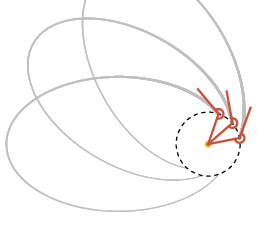
- apsidal precession: Gradual rotation of an orbit’s line of apsides (perihelion–aphelion line) due to perturbations. "Planetary perturbations can cause meteoroid orbits to precess in both argument of pericenter (apsidal precession) and longitude of ascending node"
- argument of pericenter: Orbital element specifying the angle from the ascending node to perihelion within the orbital plane. "Planetary perturbations can cause meteoroid orbits to precess in both argument of pericenter (apsidal precession) and longitude of ascending node"
- Bonferroni correction: A multiple-comparisons adjustment that divides the overall significance level across tests to control Type I error. "This is known as the Bonferroni correction, and, at a minimum, should be applied when conducting multiple tests on a single data set."
- chi-squared distribution: A probability distribution used for goodness-of-fit and nested model comparisons, among other tests. "where is the inverse CDF of a chi-squared distribution (with, in this case, 2 degrees of freedom)."
- cumulative distribution function (CDF): A function giving the probability that a random variable is less than or equal to a value. "where is the inverse cumulative distribution function (CDF) of a standard normal distribution"
- dummy variable: A binary indicator variable used to encode categorical conditions in regression models. "We separate 2026 from the rest of the data by introducing a dummy variable, , that is equal to one for fireballs observed in 2026 and zero in all other cases."
- Fisher's exact test: An exact test for independence in contingency tables, appropriate for small counts. "we use Fisher's exact test for a difference in proportions \citep{fisher22,agresti13} rather than a chi-squared test."
- generalized linear models (GLMs): A flexible class of models linking the mean of a response to predictors via a link function and a specified distribution. "The reader may not be aware, however, that linear regression is a member of a larger family of generalized linear models (GLMs)."
- geocentric (radiant): A meteor radiant corrected for Earth’s gravity (as opposed to the apparent radiant). "it is not clear whether these radiants are apparent or geocentric \citep[i.e., corrected for Earth's gravity;] []{gural01}."
- homoskedasticity: The property that residual variance is constant across levels of predictors. "display a constant variance (homoskedasticity), and"
- identity link function: A GLM link where the mean of the response equals the linear predictor without transformation. "We have chosen a Poisson model with an identity link function."
- interaction (in regression): A modeling term allowing the effect of one predictor to depend on another. "which is accomplished by allowing to ``interact'' with ."
- Kolmogorov-Smirnov (K-S) test: A nonparametric test comparing distributions; the 2D, two-sample version compares spatial distributions. "We performed a two-sample, two-dimensional Kolmogorov-Smirnov (K-S) test \citep{fasano87} on the radiant distribution."
- link function: The function that relates the expected value of the response to the linear predictor in a GLM. "where is known as the link function."
- logit: A link/quantile function defined as the inverse of the logistic CDF, often used for binomial GLMs. "The
logit'' andprobit'' functions are the quantile functions of the logistic and normal distributions, respectively." - longitude of ascending node: The angle from a reference direction to the ascending node of an orbit. "and longitude of ascending node \citep[nodal precession; see] [for Taurid precession rates]{asher93}."
- nodal precession: The slow rotation of an orbit’s line of nodes due to perturbations, shifting intersection timing with Earth. "longitude of ascending node \citep[nodal precession; see] [for Taurid precession rates]{asher93}."
- ordinary least squares (OLS): The standard linear regression method minimizing the sum of squared residuals. "The reader is almost certainly familiar with linear regression performed via ordinary least squares (OLS),"
- overdispersion: Variance exceeding the mean under a Poisson assumption, often indicating model misspecification or unobserved heterogeneity. "if the data have a larger variance than this, it can indicate either a lack of fit or overdispersion."
- Pearson residuals: Standardized residuals computed by dividing raw residuals by their expected standard deviation. "The Pearson residuals can also be used to identify outliers."
- Poisson regression: A GLM for count data where the response is modeled as Poisson-distributed around a mean linked to predictors. "Poisson regression can be used to model the rate at which events occur, if these events satisfy certain assumptions."
- probit: A link/quantile function equal to the inverse normal CDF, used for binomial-type GLMs. "The
logit'' andprobit'' functions are the quantile functions of the logistic and normal distributions, respectively." - quasi-Poisson regression: A GLM variant allowing for overdispersion by scaling the variance while keeping Poisson mean structure. "If the data appear to fit the model but overdispersion is present, quasi-Poisson regression can be used."
- quantile residuals: Residuals obtained by mapping the CDF of observed counts through an inverse normal CDF to assess departures from the model. "One alternative is to use quantile residuals:"
- radiant (meteor radiant): The point in the sky from which meteors in a shower appear to originate. "any analysis of the distribution of meteor radiants should be conducted using SCE coordinates."
- residual degrees of freedom: The number of observations minus the number of fitted parameters; used in model diagnostics. "the residual deviance will be comparable to the number of residual degrees of freedom (the number of observations minus the number of fitted parameters)."
- residual deviance: A GLM goodness-of-fit measure comparing the fitted model to a saturated model; used to check dispersion/fit. "Excess variance can be diagnosed using the residual deviance:"
- solar longitude: The Sun’s ecliptic longitude used as a proxy for time of year in meteor studies. "Points are color-coded by solar longitude (i.e., time of year)."
- sporadic sources: Non-shower background sources of meteors that contribute to a diffuse radiant distribution. "variations in background radiant density due to the sporadic sources in SCE coordinates."
- Sun-centered ecliptic (SCE) coordinates: A non-inertial coordinate system aligned with the ecliptic and Sun–Earth vector for analyzing meteor radiants. "we call these coordinates Sun-centered ecliptic (SCE) coordinates."
- Sun-Earth-radiant angle: The angle between the Sun–Earth line and the incoming meteoroid direction; conserved under nodal precession. "Nodal precession also preserves the Sun-Earth-radiant angle (see Fig.\,\ref{fig:sce})."
- two-tailed test: A hypothesis test that considers extreme deviations in both directions from the null. "outlier identification is generally a two-tailed test."
- weighted least squares: A regression method that weights observations by the inverse of their variance, useful when variances differ. "One can then perform weighted least squares, or unweighted OLS after regularizing the data"
Collections
Sign up for free to add this paper to one or more collections.