Approximating Peak Prevalence in Multistage SIR Epidemics

Abstract: Estimating peak prevalence is a central problem in epidemic modeling because it determines the period of greatest infectious burden and is closely linked to health-care demand. In multistage SIR models, however, peak prevalence is generally less tractable than in the classical model with exponentially distributed infectious periods. Motivated by the use of weighted infectious-stage aggregates as surrogates for prevalence, we investigate the relationship between the prevalence peak and the maximum of a weighted stage functional in deterministic SI$(k)$R epidemic models. We show that this relationship depends critically on how the stage-progression rate is scaled as the number of infectious stages increases. Under naive scaling, in which the progression rate remains fixed, the weighted peak is asymptotically equivalent to the prevalence peak and the commonly used factor-two approximation fails. Under Erlang scaling, which preserves the mean infectious period, the multistage model converges to a delay formulation in which prevalence and the weighted stage functional become unweighted and triangularly weighted moving averages of incidence. This limiting representation provides a theoretical basis for the factor-two approximation and identifies the regimes in which it is accurate. It also explains why this approximation deteriorates as epidemic waves become more sharply peaked. We derive analytical error bounds and develop curvature-based and parameter-based corrections that substantially improve accuracy. Numerical studies confirm these improvements across a broad range of epidemiological parameters. Overall, the results show when weighted-stage peaks can be used reliably as proxies for peak prevalence and how the resulting estimates can be refined when the standard approximation loses accuracy.

• The paper formulates a relationship between peak prevalence and weighted-stage aggregates in SI(k)R models, challenging the traditional factor-two heuristic.
• It rigorously analyzes both naive and Erlang scaling regimes, deriving explicit conditions and corrections that relate prevalence to easily measurable incidence data.
• The study introduces higher-order corrections that ensure less than 5% error, offering practical guidelines for epidemic forecasting in high-R0 scenarios.

Approximating Peak Prevalence in Multistage SIR Epidemics

Problem Formulation and Motivation

This paper rigorously investigates the relationship between peak prevalence and weighted-stage aggregates within the SI$(k)$R framework, particularly under different scaling regimes for stage progression rates. The core motivation is practical: direct observation of prevalence is often infeasible due to limitations in healthcare surveillance, driving the demand for analytic proxies based on readily accessible incident case data. The authors focus on deterministic multistage SIR models, parameterized by $k$ infectious stages, moving beyond the classical SIR (exponential infectious periods) to address realistic non-exponential dwell times.

The SI$(k)$R ODE system analyzed is

$$\begin{aligned} \dot{S}^{(k)} &= -\beta S^{(k)} I^{(k)} \ \dot{I}_1^{(k)} &= \beta S^{(k)} I^{(k)} - \delta I^{(k)}_1 \ \dot{I}_i^{(k)} &= \delta I^{(k)}_{i-1} - \delta I^{(k)}_i, \;\; i = 2,\dots,k \ \dot{R}^{(k)} &= \delta I^{(k)}_k \end{aligned}$$

with the total prevalence $I^{(k)}(t) = \sum_{i=1}^k I_i^{(k)}(t)$ and the aggregate weighted functional

$V^{(k)}(t) = \sum_{i=1}^{k}(k-i+1)I_i^{(k)}(t).$

The normalized version $W^{(k)}(t) = V^{(k)}(t)/k$ serves as the focal analytic surrogate for prevalence, with the goal to characterize the regimes in which $W^{(k)}_{\max}$ reliably approximates $I^{(k)}_{\max} = \max_t I^{(k)}(t)$.

Scaling Regimes and Analytical Results

Two distinct asymptotic regimes are studied: naive scaling (fixed per-stage rate $\delta$ as $k$0) and Erlang scaling ($k$1, so mean infectious period is fixed as $k$2 increases).

Naive Scaling

Under naive scaling, the infectious population concentrates at the start of the chain, yielding to leading order: $k$3 as $k$4. This directly refutes the widely used factor-two heuristic ($k$5) in this regime. Analytical bounds are precisely derived for $k$6 as functions of $k$7, $k$8, $k$9, and initial condition $(k)$0.

Erlang Scaling

By contrast, under Erlang scaling, the process admits a delay differential equation limit, with prevalence and the weighted-stage functional converging, respectively, to a moving average and a triangularly weighted moving average of incidence over the infectious period: $(k)$1 where $(k)$2 denotes incidence and $(k)$3 the infectious period. Under broad incidence peaks, Laplace asymptotics confirm: $(k)$4 and provide explicit conditions for the validity of this approximation.

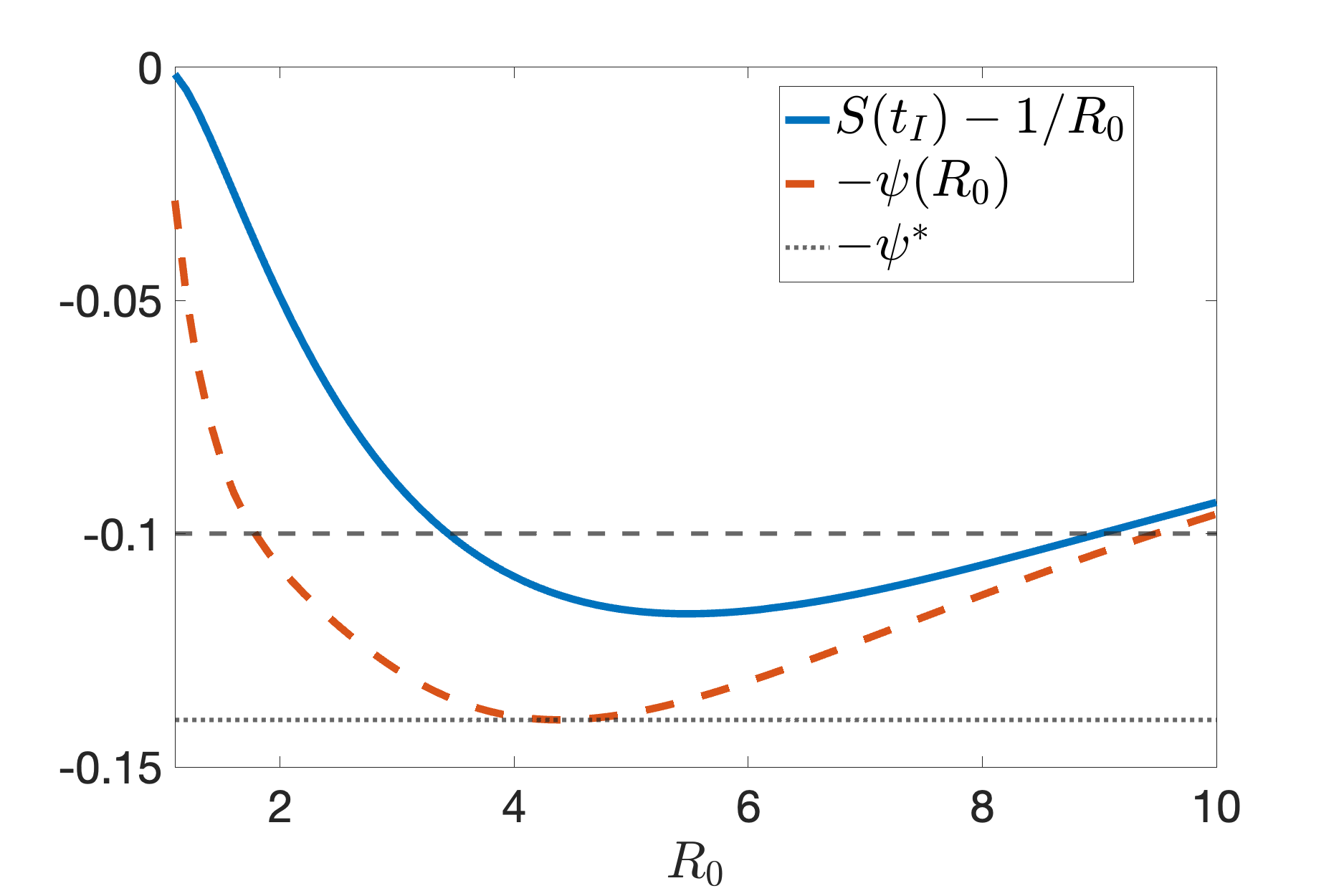
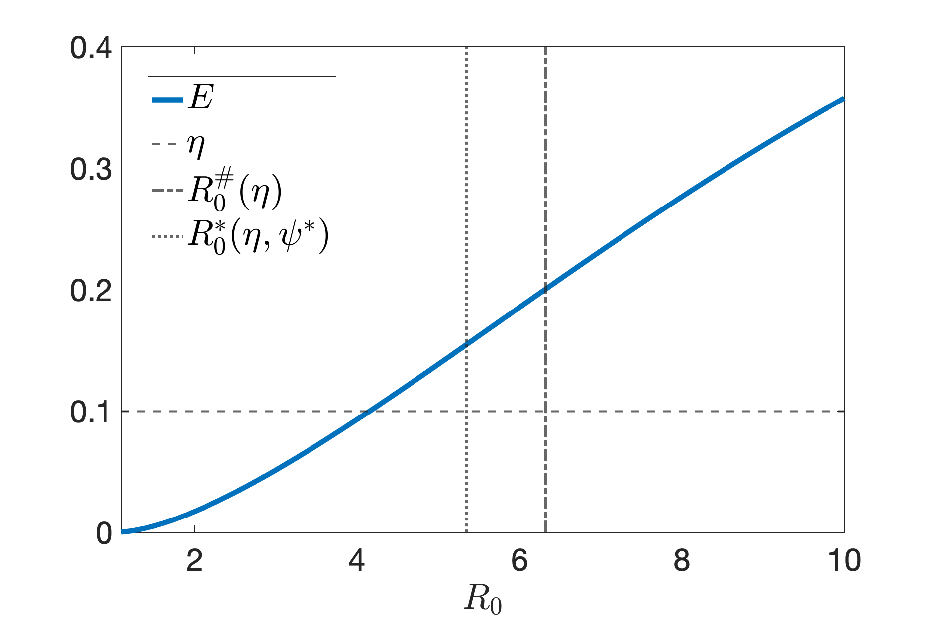
Figure 1: Analytical and numerical constraints on the accuracy of the approximation $(k)$5.

Accuracy of the Factor-Two Approximation and Corrections

The core analytical insight is that $(k)$6 is valid specifically when the relative width of the incidence peak, parameterized by $(k)$7 (with $(k)$8 the local curvature of $(k)$9 at its maximum), is small. For sharper, high-$$\begin{aligned} \dot{S}^{(k)} &= -\beta S^{(k)} I^{(k)} \ \dot{I}_1^{(k)} &= \beta S^{(k)} I^{(k)} - \delta I^{(k)}_1 \ \dot{I}_i^{(k)} &= \delta I^{(k)}_{i-1} - \delta I^{(k)}_i, \;\; i = 2,\dots,k \ \dot{R}^{(k)} &= \delta I^{(k)}_k \end{aligned}$$0 outbreaks, the relative error

$$\begin{aligned} \dot{S}^{(k)} &= -\beta S^{(k)} I^{(k)} \ \dot{I}_1^{(k)} &= \beta S^{(k)} I^{(k)} - \delta I^{(k)}_1 \ \dot{I}_i^{(k)} &= \delta I^{(k)}_{i-1} - \delta I^{(k)}_i, \;\; i = 2,\dots,k \ \dot{R}^{(k)} &= \delta I^{(k)}_k \end{aligned}$$1

increases and explicit necessary conditions on $$\begin{aligned} \dot{S}^{(k)} &= -\beta S^{(k)} I^{(k)} \ \dot{I}_1^{(k)} &= \beta S^{(k)} I^{(k)} - \delta I^{(k)}_1 \ \dot{I}_i^{(k)} &= \delta I^{(k)}_{i-1} - \delta I^{(k)}_i, \;\; i = 2,\dots,k \ \dot{R}^{(k)} &= \delta I^{(k)}_k \end{aligned}$$2 for a fixed error tolerance are derived.

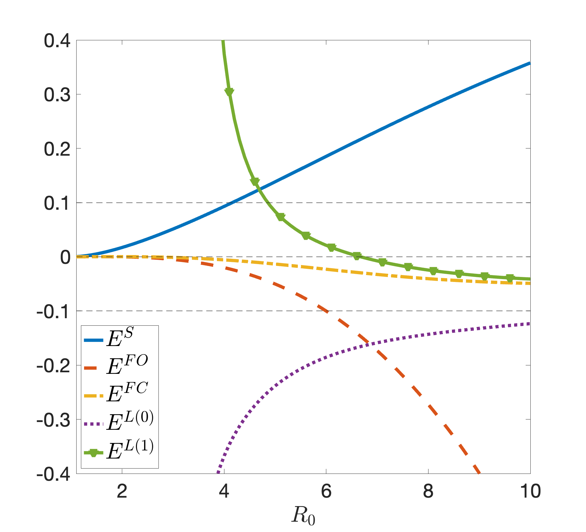
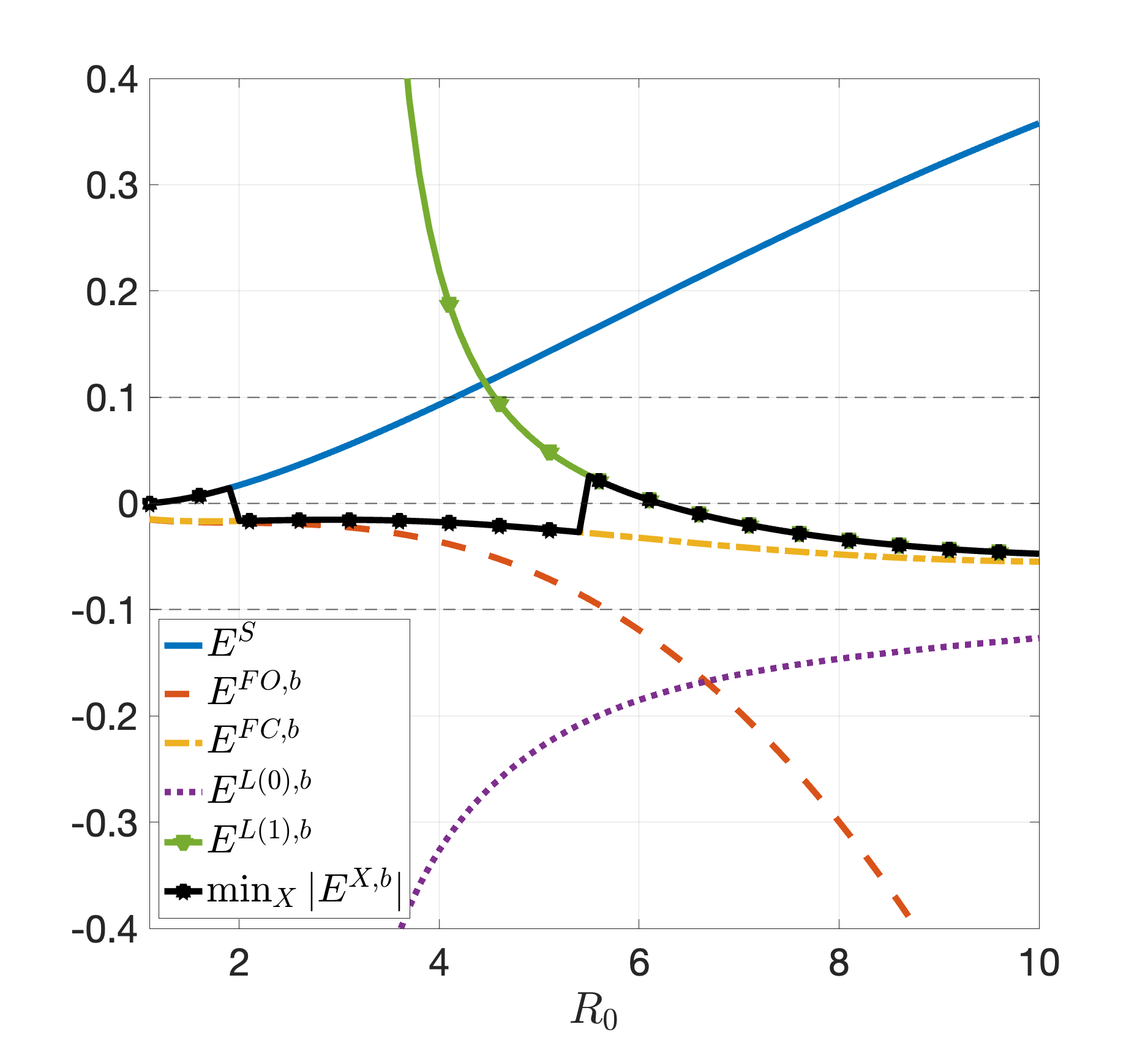
Figure 2: Relative errors $$\begin{aligned} \dot{S}^{(k)} &= -\beta S^{(k)} I^{(k)} \ \dot{I}_1^{(k)} &= \beta S^{(k)} I^{(k)} - \delta I^{(k)}_1 \ \dot{I}_i^{(k)} &= \delta I^{(k)}_{i-1} - \delta I^{(k)}_i, \;\; i = 2,\dots,k \ \dot{R}^{(k)} &= \delta I^{(k)}_k \end{aligned}$$3 of different approximations of $$\begin{aligned} \dot{S}^{(k)} &= -\beta S^{(k)} I^{(k)} \ \dot{I}_1^{(k)} &= \beta S^{(k)} I^{(k)} - \delta I^{(k)}_1 \ \dot{I}_i^{(k)} &= \delta I^{(k)}_{i-1} - \delta I^{(k)}_i, \;\; i = 2,\dots,k \ \dot{R}^{(k)} &= \delta I^{(k)}_k \end{aligned}$$4 as functions of $$\begin{aligned} \dot{S}^{(k)} &= -\beta S^{(k)} I^{(k)} \ \dot{I}_1^{(k)} &= \beta S^{(k)} I^{(k)} - \delta I^{(k)}_1 \ \dot{I}_i^{(k)} &= \delta I^{(k)}_{i-1} - \delta I^{(k)}_i, \;\; i = 2,\dots,k \ \dot{R}^{(k)} &= \delta I^{(k)}_k \end{aligned}$$5.

To extend accuracy to regimes where the factor-two rule fails, a hierarchy of higher-order corrections is constructed:

• First-order correction:

$$\begin{aligned} \dot{S}^{(k)} &= -\beta S^{(k)} I^{(k)} \ \dot{I}_1^{(k)} &= \beta S^{(k)} I^{(k)} - \delta I^{(k)}_1 \ \dot{I}_i^{(k)} &= \delta I^{(k)}_{i-1} - \delta I^{(k)}_i, \;\; i = 2,\dots,k \ \dot{R}^{(k)} &= \delta I^{(k)}_k \end{aligned}$$6

• Fully corrected (FC) and large-$$\begin{aligned} \dot{S}^{(k)} &= -\beta S^{(k)} I^{(k)} \ \dot{I}_1^{(k)} &= \beta S^{(k)} I^{(k)} - \delta I^{(k)}_1 \ \dot{I}_i^{(k)} &= \delta I^{(k)}_{i-1} - \delta I^{(k)}_i, \;\; i = 2,\dots,k \ \dot{R}^{(k)} &= \delta I^{(k)}_k \end{aligned}$$7 approximations (L(1)): explicit expressions in terms of $$\begin{aligned} \dot{S}^{(k)} &= -\beta S^{(k)} I^{(k)} \ \dot{I}_1^{(k)} &= \beta S^{(k)} I^{(k)} - \delta I^{(k)}_1 \ \dot{I}_i^{(k)} &= \delta I^{(k)}_{i-1} - \delta I^{(k)}_i, \;\; i = 2,\dots,k \ \dot{R}^{(k)} &= \delta I^{(k)}_k \end{aligned}$$8 only, derived from the curvature and model parameters, maintain absolute relative errors $$\begin{aligned} \dot{S}^{(k)} &= -\beta S^{(k)} I^{(k)} \ \dot{I}_1^{(k)} &= \beta S^{(k)} I^{(k)} - \delta I^{(k)}_1 \ \dot{I}_i^{(k)} &= \delta I^{(k)}_{i-1} - \delta I^{(k)}_i, \;\; i = 2,\dots,k \ \dot{R}^{(k)} &= \delta I^{(k)}_k \end{aligned}$$9 across broad parameter ranges.

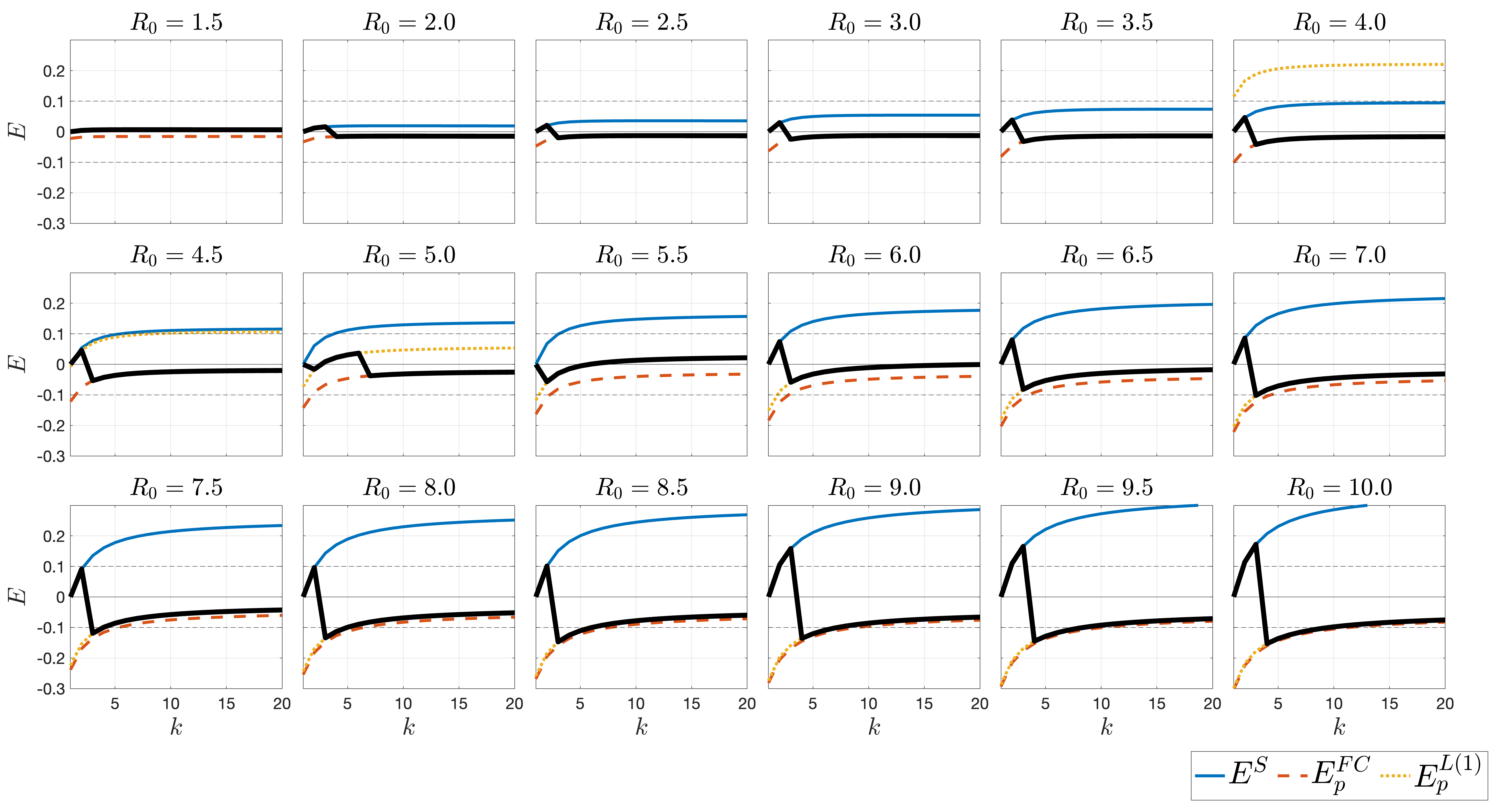
  Figure 3: Relative errors of approximations of $I^{(k)}(t) = \sum_{i=1}^k I_i^{(k)}(t)$0 as $I^{(k)}(t) = \sum_{i=1}^k I_i^{(k)}(t)$1 varies for different $I^{(k)}(t) = \sum_{i=1}^k I_i^{(k)}(t)$2.

  

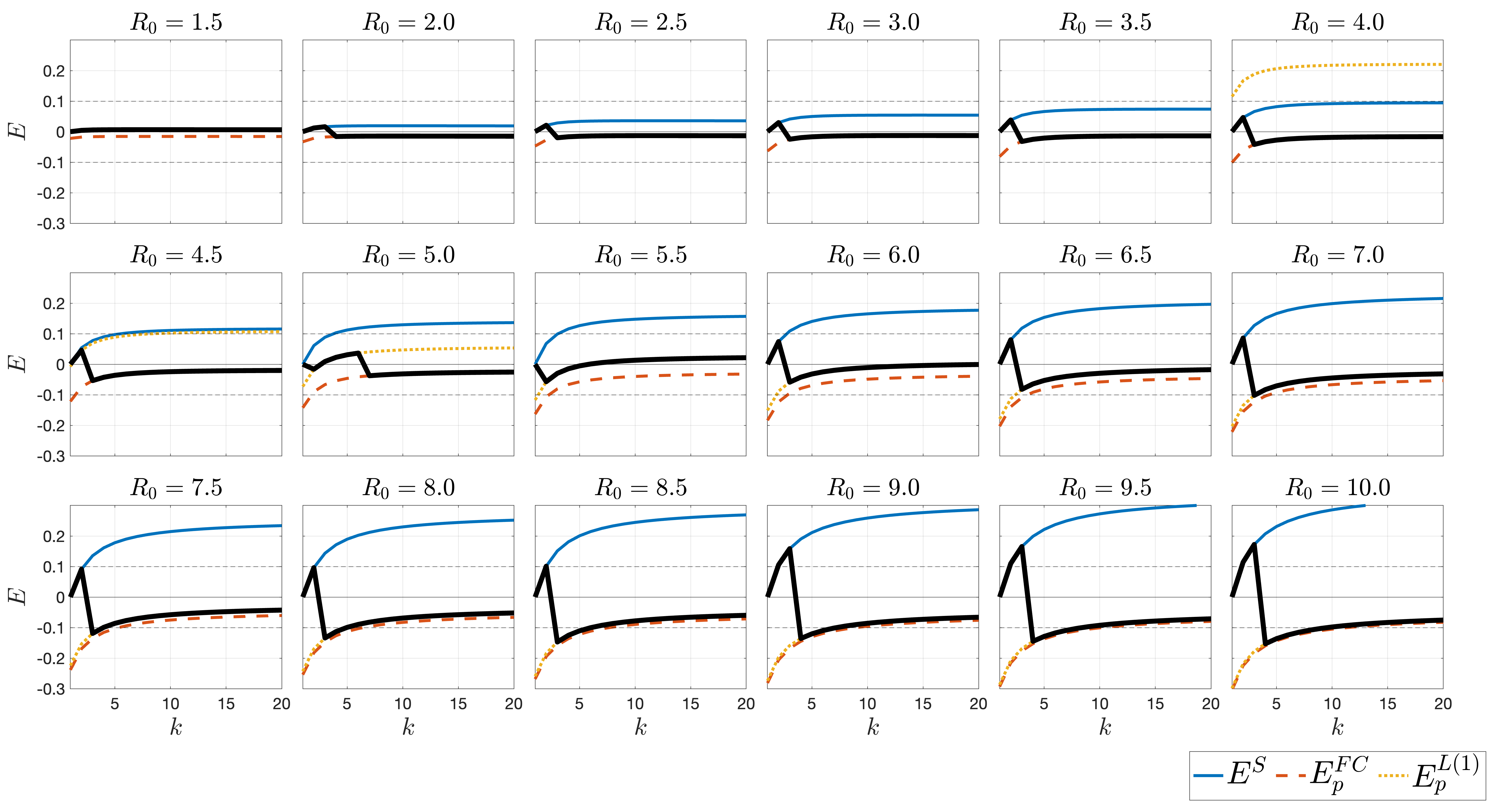
  Figure 4: Relative errors of parameter-based (plug-in) approximations for finite $I^{(k)}(t) = \sum_{i=1}^k I_i^{(k)}(t)$3 and varying $I^{(k)}(t) = \sum_{i=1}^k I_i^{(k)}(t)$4.

Numerical studies validate that for practical situations (epidemiologically relevant $I^{(k)}(t) = \sum_{i=1}^k I_i^{(k)}(t)$5), the appropriately corrected surrogate peaks (FO, FC, $I^{(k)}(t) = \sum_{i=1}^k I_i^{(k)}(t)$6) yield robust estimates of $I^{(k)}(t) = \sum_{i=1}^k I_i^{(k)}(t)$7.

Practical and Theoretical Implications

The paper has several notable implications:

• For epidemic forecasting, weighted incidence functionals, computed from easier-to-measure incidence data, can reliably estimate peak infectious burden—but only with scaling and correction formulas suited to the underlying compartmental structure.
• For mathematical epidemiology, the SI$I^{(k)}(t) = \sum_{i=1}^k I_i^{(k)}(t)$8R limit bridges finite Markovian models and age-of-infection renewal equations, clarifying how incidence and prevalence relate as time-averaged quantities with different kernel shapes.
• The corrections and bounds derived here are essential for accurate estimation in high-$I^{(k)}(t) = \sum_{i=1}^k I_i^{(k)}(t)$9, sharp-peak scenarios, as encountered in rapidly spreading epidemics.
• The theoretical framework may be extended to more general dwell time distributions, heterogeneous contact networks, or partially observed processes.

Conclusion

This work provides a comprehensive asymptotic and numerical analysis of prevalence peak estimation in multistage SIR models, resolving longstanding confusion regarding the factor-two rule and developing a suite of improved surrogate approximations for practical use. The structure-function relationship between prevalence and weighted incidence, as elucidated here, supplies essential methodology for epidemic risk assessment in settings where true prevalence data are unavailable (2607.01014).