Neural Scaling Universality: If Exponents Are Fixed, Time to Understand Coefficients
Abstract: Neural scaling laws describe how pre-training loss decays as power laws with training time, model size, and compute. This position paper argues that the exponents of these power laws are fixed by generic mechanisms: a one-third time scaling due to the strong nonlinearity of Softmax, an inverse width scaling due to representational superposition, and an inverse depth scaling due to ensemble averaging of Transformer layers. These mechanisms are robust to a wide range of data structures and architectural details, placing current LLMs in a universality class with fixed exponents. The coefficients, however, are expected to be sensitive to data and architecture details, and directly determine practical quantities such as the optimal model shape and the compute-optimal frontier. We therefore argue that understanding the coefficients is the key to near-term performance improvements, and that a closer examination of the current universality class may reveal pathways to better universality classes.
Paper Prompts
Sign up for free to create and run prompts on this paper using GPT-5.
Top Community Prompts
Explain it Like I'm 14
What is this paper about?
This paper tries to explain a big pattern seen when training LLMs: as you give models more training steps, bigger sizes, and more compute, their mistakes (called “loss”) go down in a very predictable way. The authors argue that the shapes of these curves are mostly fixed by a few simple, general reasons built into how today’s models work. What really changes from model to model are the constants in front—the “coefficients”—and those constants are the key to making practical improvements.
What questions are the authors asking?
- Why do LLMs get better with more training in a way that follows smooth “power laws” (like “loss falls roughly as one-third power of training time”)?
- Are these power-law rates mostly determined by the data we use, or by general features of the models and training methods?
- If the overall rates are fixed, what can we still tune to make models better for the same compute? In other words, what do the “coefficients” control in practice?
How did they study it? (In everyday language)
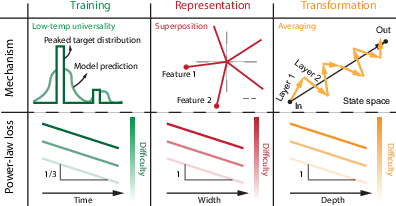
The authors combine simple, general ideas about how Transformers learn with measurements from real model families (like Pythia, Chinchilla, and Farseer). They focus on three parts of training:
- Training time effect: Softmax’s “spotlight”
- Softmax is a function that turns scores into probabilities so the model can choose the next word.
- When the correct answer is very likely (a “peaked” distribution), Softmax acts like a strong spotlight that makes training progress slow down in a specific, predictable way.
- Result: As training time increases, loss falls roughly like “one over the cube root of time” (a one-third power).
- Model width effect: Packing too many ideas into too few slots
- “Width” is like how wide the model’s representation is (think: how many “slots” or dimensions the model has to store features).
- Models try to store many more features than they have perfect space for, so different features interfere—this is called “superposition”.
- Result: The leftover error from limited width shrinks like “one over width”.
- Model depth effect: Many layers average out errors
- “Depth” is how many layers the model has.
- Layers often make similar small improvements; it’s like having many judges average their opinions to reduce errors.
- Result: The leftover error from limited depth shrinks like “one over depth”.
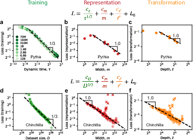
They then fit real training data using these fixed “exponents” (the one-third in time, one-over-width, one-over-depth) and let only the coefficients (the constants in front) adjust to the data. The fits work well across several model families.
What did they find, in simple terms?
- Fixed exponents from general mechanisms:
- Training time: Loss falls about as 1/(time)1/3 because Softmax becomes very nonlinear when predictions are sharp.
- Width: Leftover error falls like 1/width because features share limited space and interfere.
- Depth: Leftover error falls like 1/depth because layers collectively average away errors.
- Data vs. steps: Step-limited, not data-limited
- In large-scale “online” training, more steps usually means more data, so you also see loss fall about as 1/(dataset size)1/3.
- The authors argue the fundamental driver is steps/optimization time, not simply having endless unique data. Once your dataset is big and diverse enough, taking more steps (even with reuse) can keep improving the model.
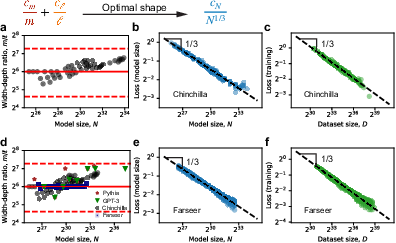
- Putting width and depth together → a one-third model-size law
- When you choose a good balance of width and depth, the total model-size effect follows a one-third power law: loss falls like 1/(model size)1/3.
- The “best” shape (how wide vs. how deep) depends on the coefficients for width and depth. Near that balance, changing shape a bit doesn’t hurt much—so practitioners don’t need to tune it perfectly.
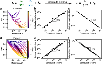
- Compute-optimal planning
- If you fix your total compute budget, there’s a best trade-off between model size (parameters) and data (tokens). Theory says the best ratio depends on the coefficients.
- At this best trade-off, loss improves with compute as 1/(compute)1/6, and both model size and dataset size grow like the square root of compute.
- Coefficients matter for real-world design
- The exponents (like “one-third”) look universal for today’s LLMs, but the coefficients vary with architecture, optimizer, and data choices.
- Those coefficients set practical recipes: the best width-to-depth ratio, the best tokens-per-parameter ratio, and how fast loss falls per extra token or FLOP.
- Evidence across model families
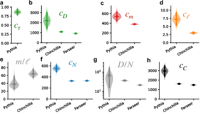
- Using Pythia, Chinchilla, and Farseer data, the authors show the fixed-exponent fits work well and the inferred coefficients differ in sensible ways across families.
- Alternative views exist
- Other theories say the power laws come mainly from patterns in the data (like how often different skills appear) and predict exponents that vary with the data.
- The authors suggest both worlds might apply at different stages: early training may reflect data patterns, while later training is dominated by the Softmax-driven “universality” they describe.
Why is this important?
- Clear rules of thumb: If the exponents are “locked in” by the model’s general behavior, we don’t need to chase different exponents for every dataset. Instead, we focus on the coefficients that we can change with better architecture, optimizers, or data curation.
- Smarter model design: Knowing how width and depth contribute lets you choose a good shape without endless trial and error.
- Better use of compute: The coefficients tell you how to split your budget between model size and training tokens to get the best results.
- Practical path to gains now: Tweaking learning rate schedules, batch sizes, or optimizers can improve “loss per token” by improving the relevant coefficients—even if the exponents stay the same.
Key terms explained
- Loss: A number that measures how wrong the model’s predictions are. Lower is better.
- Power law: A pattern like “loss falls as the one-third power of time,” meaning if you multiply time by 8, loss shrinks by about 2 (since 81/3 = 2).
- Exponent vs. coefficient:
- Exponent: The power in a power law (like the “one-third”). Think of it as the curve’s shape.
- Coefficient: The constant in front that shifts the curve up or down. Think of it as a dial that speeds up or slows down progress without changing the shape.
- Softmax: A function that turns raw scores into probabilities; when one answer is much better than the rest, it acts like a strong spotlight on that answer.
- Width: Roughly, how many “slots” the model has to store features (embedding dimension).
- Depth: How many layers the model has.
- Universality (in this paper): The idea that different models and datasets can show the same scaling shapes (the same exponents) because they share the same basic mechanisms, even if their coefficients differ.
Bottom line
- The authors argue that today’s LLMs fall into a “universality class” where the main scaling rates—the exponents—are fixed by general mechanisms: Softmax’s strong nonlinearity (time), representation interference (width), and layer averaging (depth).
- The constants in front—the coefficients—depend on choices you can control, like architecture, optimizer, and data setup. Those coefficients determine the best shape of the model, the best token-to-parameter ratio, and the best loss you can get for a given compute budget.
- So, if exponents are fixed, the fastest way to better models is to understand and improve the coefficients.
Knowledge Gaps
Knowledge gaps, limitations, and open questions
Below is a consolidated list of concrete gaps and open questions the paper leaves unresolved. Each point highlights what is missing, uncertain, or left unexplored, and is intended to guide actionable follow-up studies.
- Universality claim validation: Lack of broad, prospective validation that the exponents {time: 1/3, width: −1, depth: −1} hold across diverse model families, scales (beyond Pythia/Chinchilla/Farseer), and training regimes.
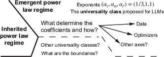
- Boundaries of the universality class: No formal criteria for when the proposed class applies versus data-driven exponent regimes; no diagnostics to detect regime transitions during training.
- Softmax/low-entropy assumption: Unclear quantitative “low-temperature/low-entropy” threshold at which the 1/3 time exponent emerges, and how/when training transitions from a “high-temperature” (data-sensitive) to “low-temperature” (universal) regime.
- Objective-function dependence: Unverified whether the exponents persist for non-Softmax or mixed objectives (e.g., contrastive, masked LM, MSE, RL, RLHF, auxiliary losses).
- Modality and task generality: No evidence the exponents and decomposition hold for vision, speech, RL, multimodal, or retrieval-augmented settings.
- Additive separability of loss: The asserted additive form L ≈ c_τ/τ{1/3} + c_m/m + c_ℓ/ℓ + L0 lacks a rigorous derivation and quantification of cross-terms or interaction corrections at finite scale.
- Finite-size/early-training corrections: Missing characterization of non-asymptotic regimes, cross-over behavior, and the practical ranges (m, ℓ, τ, D) where asymptotic scaling becomes reliable.
- Mapping from tokens to dynamic time: The relation D ∝ τ (and c_D as a function of c_τ, η, B, schedule) is asserted but not quantified across optimizers, schedules (warmup/decay/restarts), and batch-size scaling rules.
- Step-limited vs data-limited: The claim that pre-training is step-limited (not fundamentally data-limited) is not experimentally demonstrated under controlled data reuse, deduplication levels, and distribution-shift conditions.
- Optimizer dependence: No predictive framework linking c_τ (and via it c_D) to optimizer class (AdamW, Muon, Shampoo, etc.), momentum/adaptivity, preconditioning strength, and gradient-noise scale.
- Batch-size and learning-rate scaling: The heuristic η ∝ √B and its implications for c_D and D–τ mapping lack systematic empirical validation across large hyperparameter grids and schedule shapes.
- Estimating and interpreting L0: Methods to estimate the irreducible loss L0 robustly are not specified; its dependence on tokenization, evaluation distribution, and domain composition is unclear.
- Coefficient identifiability: Current datasets are insufficient to disentangle c_m from c_ℓ cleanly (e.g., Farseer degeneracy m ∝ ℓ); requires factorial sweeps that vary width and depth independently at fixed N and/or C.
- Stability of coefficient estimates: Bootstrap intervals are wide; no standardized measurement protocol for c_τ, c_m, c_ℓ (and derived c_N, c_D, c_C) across labs, tasks, and datasets.
- Superposition mechanism tests: The inverse-width claim (c_m/m) is not backed by direct measurements of representational interference versus m, nor tests of interventions meant to reduce superposition (e.g., sparse coding, orthogonality constraints) and observe predicted coefficient/exponent changes.
- Depth-as-ensemble mechanism tests: No causal experiments that manipulate layer similarity (e.g., weight tying, layer reordering, disabling residuals) to validate the ensemble-averaging explanation and to probe the conditions for ℓ{-1} vs ℓ{-3}.
- Architectural boundary conditions: No systematic exploration of whether MoE, recurrence/SSMs, linear attention, normalization variants, activation functions, or looped/ARNet designs change coefficients only (as hypothesized) or also exponents.
- Sequence-length and context effects: Absent analysis of how scaling and coefficients depend on sequence length/context window (e.g., at very long contexts or with length curricula).
- Compute accounting fidelity: The compute proxy C ≈ 6ND ignores optimizer overheads, activation checkpointing, sequence-length variability, memory bandwidth effects, and MoE routing costs; implications for “compute-optimal” scaling may be distorted.
- Generality of one-sixth compute scaling: One-sixth exponent at the compute-optimal frontier is shown only for limited ranges; no tests at substantially larger compute or different training recipes to check for phase changes.
- Downstream capability linkage: No evidence that fixed exponents or improved coefficients in pre-training loss translate systematically to gains in downstream tasks (zero/few-shot, math, code, reasoning, calibration).
- Data quality and composition: No operational definition or metric connecting data quality/diversity to c_τ and c_D; unclear how deduplication, curriculum, domain mixing, and contamination alter coefficients and optimal ratios.
- Tokenizer and vocabulary effects: Unexplored impact of tokenizer choice and vocabulary size on L0, c_m, and overall scaling behavior.
- Multilingual and domain dependence: Lack of coefficient/exponent measurements across languages and high-entropy domains (e.g., morphologically rich languages, code, math) to test robustness of the low-entropy assumption.
- Regularization impacts: Effects of label smoothing, dropout, weight decay, and gradient clipping on both exponents and coefficients are not characterized.
- Interaction with parameter sharing/weight tying and quantization: Unclear whether tying/adapter schemes or quantization change exponents or only coefficients.
- Online coefficient estimation: No method proposed to estimate c_τ, c_m, c_ℓ on-the-fly during training to steer aspect ratio, D/N, and schedule adaptively.
- Regime diagnostics: No practical indicators (e.g., output entropy, gradient norms) to detect entry into the universality regime or to forecast cross-over points.
- Data reuse and memorization risks: The step-limited claim does not address overfitting/memorization when reusing tokens, nor how these risks alter coefficients or asymptotic exponents.
- Robustness of reconstructed datasets: Fits rely partly on reconstructed Chinchilla curves; the impact of reconstruction error on inferred coefficients/exponents is not quantified.
- Universality class mapping: No roadmap to discover additional universality classes, nor controlled experiments to chart boundaries and transition mechanisms between classes.
- Fine-tuning/RLHF phases: Unclear whether the proposed exponents/coefficients persist through instruction-tuning and RLHF, or how pre-train coefficients predict post-train efficiency and outcomes.
- Practical design guidance completeness: While aspect-ratio and D/N prescriptions depend on coefficients, concrete procedures to set them under realistic hardware/throughput/memory constraints are not provided.
Practical Applications
Immediate Applications
The paper’s fixed-exponent view (time: one‑third, width: inverse‑width, depth: inverse‑depth) and “coefficients matter” thesis enables several deployable practices now:
- Compute planning and ROI forecasting (industry: AI labs, cloud; sectors: software, finance, healthcare)
- Use C-1/6 return and N ∝ C1/2 at the compute‑optimal frontier to set training budgets, predict marginal gains, and schedule hardware procurement.
- Tools/workflows: MLOps dashboards that fit isoFLOP curves and forecast compute‑optimal points.
- Assumptions/dependencies: Training is in the asymptotic regime; fixed exponents hold; reliable estimation of c_D and c_N.
- Architecture sizing and aspect‑ratio guidelines (industry/academia; sectors: software, hardware co‑design)
- Size models near the optimal aspect ratio m/ℓ ≈ c_m/(2c_ℓ); exploit the observed flatness near optimum to reduce grid search.
- Tools/workflows: Config generators that set m and ℓ from fitted c_m, c_ℓ; design checklists enforcing m ∝ ℓ near the optimum.
- Assumptions/dependencies: Additive loss decomposition holds; layers act roughly like an ensemble (L ∼ ℓ-1); coefficients measurable on a small model sweep.
- Token/parameter allocation for fixed compute (industry; sectors: software, cloud economics)
- For given compute C, allocate tokens and parameters with D/N = (c_D/c_N)3; expect near‑linear D ∝ N at optimum.
- Tools/workflows: Training planners that set D and N jointly; procurement aligned to token pipelines and parameter count.
- Assumptions/dependencies: Online regime links data and time (D ∝ τ approximately); stable mapping from c_τ to c_D via hyperparameters.
- Hyperparameter tuning for data efficiency (industry/academia; sectors: software)
- Tune learning rate η, batch size B, and schedule shapes to maximize loss‑per‑token via the c_τ→c_D relationship (keep D ∝ τ as closely as possible).
- Tools/workflows: Auto‑tuning LR/B schedulers targeting dynamic time τ; automated detection of step‑limited under‑training.
- Assumptions/dependencies: Comparable schedule shapes across runs; known noise scaling with batch size.
- Data strategy: prioritize diversity and quality over raw volume (industry; sectors: data engineering, healthcare/finance NLP)
- Since training is step‑limited in this view, invest in deduplication, domain balance, and high‑quality pipelines rather than continually growing unique tokens.
- Tools/workflows: Dedup pipelines; sampling/mixing strategies to stabilize c_τ and reduce c_m by relieving superposition conflicts.
- Assumptions/dependencies: Target distributions become peaked (low‑entropy) during training; reusing diverse data does not degrade gradients.
- Optimizer and schedule selection by coefficient shifts (industry; sectors: software)
- Prefer methods that improve c_τ/c_D (e.g., Muon, Sophia, Shampoo variants) without relying on exponent changes; quantify speedups as coefficient multipliers.
- Tools/workflows: Side‑by‑side coefficient benchmarking; “optimizer cards” reporting changes in c_τ, c_D.
- Assumptions/dependencies: Comparable stability and convergence windows across optimizers.
- Standardized “Coefficient Cards” for model reporting (academia/industry/policy)
- Report c_τ, c_m, c_ℓ, c_D (and derived c_N, c_C) alongside exponents to enable fair cross‑family comparisons and reproducible scaling forecasts.
- Tools/workflows: Open‑source fitting scripts; leaderboards displaying coefficients and optimal m/ℓ, D/N.
- Assumptions/dependencies: Access to training curves and saturation loss across a few widths/depths.
- Energy and sustainability impact estimates (policy/industry; sectors: energy, cloud)
- Translate C-1/6 diminishing returns into carbon/energy forecasts; inform procurement and emissions targets.
- Tools/workflows: Green‑AI calculators that map coefficient‑based loss forecasts to energy and emissions.
- Assumptions/dependencies: Power usage effectiveness and hardware efficiency profiles known; compute‑optimal scaling remains valid.
- Fine‑tuning step budgeting for domain models (industry/SMBs; sectors: healthcare, finance, law)
- Use τ‑based forecasts to set steps for domain adaptation; expect returns to follow the one‑third time scaling until saturation.
- Tools/workflows: Fine‑tune monitors that estimate c_τ online and predict convergence.
- Assumptions/dependencies: Loss landscape remains in low‑temperature regime for the target task; adequate domain data diversity.
- Education and curriculum (academia)
- Lab exercises to measure c_τ, c_m, c_ℓ, demonstrate isoFLOP curves, and validate compute‑optimality.
- Tools/workflows: Teaching notebooks; small‑scale Pythia‑like suites.
- Assumptions/dependencies: Small models still display asymptotic trends sufficiently to fit coefficients.
- Cloud advisory services and pricing (industry; sectors: cloud)
- Offer “scaling advisors” that recommend N, D, and training schedules given budget and latency/throughput constraints.
- Tools/workflows: API that ingests a few pilot runs and outputs coefficient‑aware plans.
- Assumptions/dependencies: Customer workloads map to the same universality class; pilot data representative.
Long-Term Applications
The paper also suggests research and development directions that require further validation, scaling, or tooling:
- Architecture and mechanism search for better coefficients or new universality classes (industry/academia; sectors: software, hardware)
- Explore attention residual networks, MoE, looped Transformers, alternative normalizations/activations to reduce c_ℓ or c_m; seek mechanisms that alter exponents to exceed the current C-1/6 ceiling.
- Tools/workflows: NAS/AUTO-ML loops optimizing coefficients; ablation farms.
- Assumptions/dependencies: Softmax nonlinearity and superposition/ensemble mechanisms define the present class; breaking them may yield new exponents.
- Token‑efficient training via principled data reuse and active selection (industry; sectors: data platforms)
- Build replay/curriculum systems that maximize progress per step (improve c_τ) under step‑limited training; combine with dedup and domain balancing.
- Tools/workflows: Data schedulers optimizing τ‑progress; gradient variance monitors.
- Assumptions/dependencies: Online‑training approximation; stable benefits from reuse without overfitting.
- Real‑time meta‑controllers for training (industry; sectors: MLOps)
- Agents that fit coefficients on the fly and adapt m/ℓ, D/N, LR/B, and schedule to stay on the compute‑optimal frontier as compute or objectives change.
- Tools/workflows: Closed‑loop training controllers integrated with cluster schedulers.
- Assumptions/dependencies: Reliable online coefficient estimation; smooth response of training to control inputs.
- Hardware–software co‑design for coefficient gains (industry/hardware; sectors: semiconductors, systems)
- Architect memory and interconnect to reduce representational interference (c_m) and enhance layer‑wise averaging efficiency (c_ℓ); compiler passes that restructure depth/width usage.
- Tools/workflows: Kernel fusion and scheduling aimed at depth‑averaging; novel cache hierarchies.
- Assumptions/dependencies: Microarchitectural changes translate into effective c_m/c_ℓ improvements in practice.
- Cross‑modality and cross‑domain generalization (academia/industry; sectors: vision, speech, robotics)
- Test whether fixed exponents and coefficient‑driven design carry over to vision transformers, speech models, and robot policies; if so, unify compute‑optimal planning across modalities.
- Tools/workflows: Multi‑domain scaling benchmarks with coefficient reporting.
- Assumptions/dependencies: Presence of low‑entropy targets and similar nonlinearity/superposition mechanisms.
- Standards and governance based on coefficient reporting (policy/consortia)
- Define standards requiring model releases to disclose compute, tokens, and coefficients; align energy reporting and compute governance to C-1/6 returns.
- Tools/workflows: Auditable “Coefficient & Compute Cards”; third‑party verification.
- Assumptions/dependencies: Community consensus on fitting protocols and data disclosure.
- Data markets priced by coefficient impact (industry/policy; sectors: data economy)
- Value datasets by measured improvements to c_τ or c_m instead of raw token counts; incentivize diversity and domain coverage.
- Tools/workflows: Vendor evaluation frameworks measuring coefficient deltas from pilots.
- Assumptions/dependencies: Stable attribution from data additions to coefficient shifts.
- Edge and on‑device model optimization (industry; sectors: mobile/IoT)
- Derive minimal N and D to hit targets under tight C using compute‑optimal rules; co‑tune m/ℓ for latency/memory constraints.
- Tools/workflows: On‑device scaling planners; hardware‑aware aspect ratio solvers.
- Assumptions/dependencies: Scaling relations hold when quantization/pruning are applied; depth/width trade‑offs respect latency constraints.
- Regime‑shift detectors and theory‑driven diagnostics (academia/industry)
- Instruments that detect transitions from data‑sensitive (early, high‑temperature) scaling to universality (low‑temperature) and adapt training strategy accordingly.
- Tools/workflows: Monitors of output entropy and gradient norms tied to τ.
- Assumptions/dependencies: Clear empirical signatures of regime boundaries; validated thresholds.
- AI safety and capability forecasting (policy/academia)
- Use coefficient‑aware scaling to forecast capability growth under compute constraints; inform safety evaluations and funding allocation.
- Tools/workflows: Public models projecting performance vs compute with uncertainty bands.
- Assumptions/dependencies: Task performance tracks pre‑training loss reductions; transfer to downstream metrics predictable.
- Formal proofs and mechanistic understanding (academia)
- Prove the one‑third, 1/m, and 1/ℓ scalings under realistic assumptions; characterize boundaries between universality classes.
- Tools/workflows: Theory–experiment loops; canonical datasets and model suites for replicability.
- Assumptions/dependencies: Ability to isolate mechanisms (Softmax nonlinearity, superposition, ensemble averaging) in controlled settings.
Notes on general assumptions/dependencies across applications:
- Fixed exponents arise from Softmax nonlinearity (low‑entropy targets), representational superposition, and layer‑ensemble behavior; if these mechanisms are absent or altered, the class may change.
- Additive decomposition L ≈ c_τ/τ1/3 + c_m/m + c_ℓ/ℓ + L_0 is asymptotic; small models or early training may deviate.
- Online training and adequate data diversity are needed to justify D ∝ τ and step‑limited framing.
- Coefficient estimation requires enough variation in time, width, and depth to separate terms; noise or confounding can bias fits.
Glossary
- attention distributions: The probability distributions generated by the attention mechanism over possible positions or tokens. Example: "learning peaked distributions (e.g., next-token distributions and attention distributions)"
- compute-optimal frontier: The set of model/data configurations that minimize loss for a fixed compute budget. Example: "The optimal token-to-parameter ratio or compute-optimal frontier is also determined by the coefficients, at which the loss follows a one-sixth compute scaling"
- compute-optimal loss: The minimum attainable loss at the compute-optimal frontier for a given compute budget. Example: "the compute-optimal loss agrees well with the predicted scaling"
- data manifold: A conceptual low-dimensional structure that captures the geometry of data, used to reason about learning behavior. Example: "some frameworks with high-level arguments like fitting data manifold predict that loss exponents depend only on data structure"
- dataset size scaling: The empirical power-law relationship between loss and the number of training tokens. Example: "The time scaling can be transferred to dataset size scaling because large-scale pre-training is close to online, one-epoch training"
- dataset size scaling exponent: The exponent characterizing how loss decreases with dataset size in a power law. Example: "the dataset size scaling exponent of Chinchilla, $0.28$ reported in the original paper \cite{hoffmann2022chinchilla} and $0.37$ fitted from replication \cite{besiroglu2024chinchilla}, are both close to $1/3$"
- dynamic time: An integrated notion of training time weighted by the learning rate, which governs optimization dynamics. Example: "Here is the time of optimization dynamics, or dynamic time for short, related to the number of training steps via an integral over the learning rate schedule"
- embedding dimension: The width of the model’s representation space, typically the size of token embeddings. Example: "the model's ability to represent all relevant concepts in its finite width, or embedding dimension, "
- ensemble averaging: A mechanism where multiple similar components (e.g., layers) independently reduce errors, averaging to lower total error. Example: "an inverse depth scaling due to ensemble averaging of errors across Transformer layers"
- feature frequency distributions: Distributions describing how often different features occur in data; can influence learning difficulty and coefficients. Example: "Data structures, e.g., a wide range of feature frequency distributions, affecting the difficulty of learning, primarily change the coefficients"
- geometric interference: Error arising from overlapping representations when many features are packed into limited dimensions. Example: "The geometric interference among superposed representations introduces errors"
- high-temperature regime: An early training phase where outputs are relatively flat and nonlinearity is weak. Example: "In the early stage, LLMs are in the high-temperature regime, with relatively flat output distributions where nonlinearity in loss is weak"
- inverse depth scaling: A loss decrease proportional to the inverse of the number of layers. Example: "yielding the inverse-depth scaling "
- inverse width scaling: A loss decrease proportional to the inverse of the model’s width. Example: "an inverse width scaling due to geometric interference of more features than available dimensions, i.e., superposition"
- irreducible loss: The loss floor set by inherent uncertainty in the target distribution. Example: "where is the irreducible loss set by the entropy of the target distributions"
- isoFLOP curves: Curves of loss versus model size at fixed compute, used to find compute-optimal configurations. Example: "We construct isoFLOP curves, i.e., loss as a function of model size at fixed compute "
- kernel methods: Techniques that model data via kernel functions or linearized equivalents, often used to analyze scaling in simplified settings. Example: "kernel methods or effective linear models \cite{maloney2022solvable,bordelon2025feature, bordelon2021learning,lin2024scaling,bordelon2024dynamical,worschech2024analyzing,fonseca2024exactly,paquette20244+,defilippis2025scaling} trained with mean squared error (MSE)"
- low-entropy distributions: Target distributions that are highly peaked or concentrated, making Softmax highly nonlinear. Example: "When a model learns low-entropy or peaked distributions, Softmax becomes highly nonlinear"
- low-temperature expansion: An analytic approach for peaked distributions analogous to low-temperature limits in physics. Example: "which is related to low-temperature expansion and universality"
- low-temperature regime: A later training phase where outputs are peaked and Softmax nonlinearity dominates. Example: "Later, in the low-temperature regime, where output distributions become peaked and Softmax becomes strongly nonlinear, loss follows the one-third time scaling"
- mixture of experts: An architecture that routes tokens to a subset of specialized expert sub-networks. Example: "Mixture of experts \cite{fedus2022switch, clark2022unified}, looped transformers \cite{fan2024looped, prairie2026parcae}, and attention residual networks \cite{team2026attention} should not alter the three scaling laws"
- model size scaling: The relationship between loss and the total number of parameters, often as a power law. Example: "Width and depth scaling laws lead to a one-third model size scaling at the optimal aspect ratio"
- online training: A regime where each optimization step consumes new data without revisiting previous batches. Example: "In the online training regime, each additional step consumes new tokens"
- online, one-epoch training: Training that effectively uses each token once, approximating a single pass over massive data. Example: "large-scale pre-training is close to online, one-epoch training"
- one-sixth compute scaling: The predicted loss scaling exponent with compute at the compute-optimal frontier. Example: "the loss follows a one-sixth compute scaling"
- one-third time scaling: The predicted loss scaling exponent with dynamic time during training. Example: "a one-third time scaling due to Softmax nonlinearity in learning peaked distributions"
- optimal aspect ratio: The width-to-depth ratio that minimizes loss at fixed parameter count. Example: "lead to a one-third model size scaling at the optimal aspect ratio"
- optimal shape: The combined choice of width and depth (architecture shape) that minimizes loss for a given parameter budget. Example: "At the optimal shape, determined by the coefficients, width and depth scaling laws lead to a one-third model size scaling"
- optimal token-to-parameter ratio: The ratio of training tokens to parameters that minimizes loss for a fixed compute budget. Example: "The optimal token-to-parameter ratio or compute-optimal frontier is also determined by the coefficients"
- power-law loss scaling: Loss decreasing as a power function of resources like data, time, or parameters. Example: "attributes the power-law loss scaling to some power-law structures in the data"
- pre-training loss: The training objective (e.g., cross-entropy) measured during large-scale pre-training. Example: "Neural scaling laws describe how pre-training loss decays as power laws with training time, model size, and compute"
- representational superposition: Encoding more features than dimensions by overlapping them in the representation space. Example: "an inverse width scaling due to representational superposition"
- residual loss: The remaining loss due to representation or transformation limits after training. Example: "introduces errors, leading to a residual loss "
- residual network: A network with skip connections; used here to analyze depth-related error reduction. Example: "A toy residual network analysis reveals two possible regimes"
- saturation loss: The loss value after training has effectively converged given a fixed architecture and data. Example: "the saturation loss is well described by the inverse width and depth scaling"
- Softmax nonlinearity: The strong nonlinearity of the Softmax function, especially pronounced for peaked distributions. Example: "a one-third time scaling due to Softmax nonlinearity in learning peaked distributions"
- superposition: The phenomenon of multiple features sharing representational directions in limited-dimensional spaces. Example: "a phenomenon known as superposition"
- Transformer layers: The stacked layers in Transformer architectures that process and update token representations. Example: "ensemble averaging of errors across Transformer layers"
- universality: The property that certain behaviors (e.g., exponents) are insensitive to detailed data/architecture specifics. Example: "This is a form of universality, as the one-third exponent is insensitive to the details of the data distribution"
- universality class: A category of systems sharing the same fixed scaling exponents despite differing details. Example: "a universality class of neural scaling laws is defined by the set of fixed exponents"
- universality regime: The operating regime in which universality (fixed exponents) governs scaling behavior. Example: "the universality regime is most relevant to current LLMs"
Collections
Sign up for free to add this paper to one or more collections.

