Continuous Hidden Markov Models for Equity Returns: Heavy-Tail Emission Families and Regime-Conditional Value-at-Risk
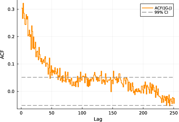
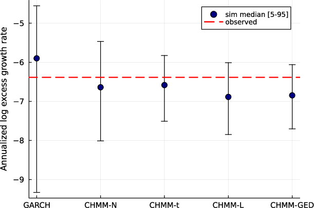
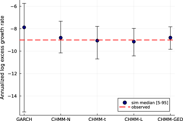
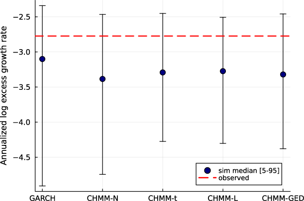
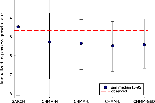
Abstract: Synthetic generators of daily equity returns let practitioners stress test, backtest, and design scenarios that a single realized market history cannot supply, but only if the generator reproduces the stylized facts of real returns: heavy tails, negligible linear autocorrelation, and slow decay of the absolute-return autocorrelation. Hidden Markov models with few Gaussian states were long thought unable to reproduce that slow decay, and the standard fix was to abandon them for more complex hidden semi-Markov models. We revisit this issue with a continuous hidden Markov model whose regime chain governs the autocorrelation while per-regime densities govern the marginal, separating the temporal and distributional sides of the original failure. A unified expectation-maximization framework fits Gaussian, Student-t, Laplace, and generalized-error emissions under shared forward-backward recursions and quantile-based initialization, and a spectral identity bounds the number of decay modes by the rank of the centred transition matrix. Across SPY walk-forward folds, a sector-balanced 30-ticker panel, a CRSP cross-decade transfer, and a six-asset basket, that bound was not binding once a few states were used: heavy-tailed marginals, not additional decay modes, closed most of the fit gap, recovering volatility clustering above the i.i.d. baseline and narrowing the kurtosis gap without a tuning hyperparameter. The original failure is therefore distributional, not temporal. On daily US equities, a simple, interpretable Markov model suffices, and unlike a bootstrap or semi-Markov fit that wins only on a single-window fit, the fitted model also yields a regime-conditional Value-at-Risk that passes a joint conditional-coverage test and a copula that reproduces cross-asset correlations: one interpretable generator serving both path simulation and downstream risk and portfolio tasks.
Paper Prompts
Sign up for free to create and run prompts on this paper using GPT-5.
Top Community Prompts
Explain it Like I'm 14
Continuous Hidden Markov Models for Equity Returns — A simple explanation
What is this paper about?
The paper builds and tests a realistic “market simulator” for daily U.S. stock returns. The simulator is based on a model that assumes markets switch between a few hidden “regimes” (like moods: calm, nervous, excited). Each regime has its own pattern for how big and how frequent ups and downs are. The goal is to generate believable fake price paths for testing strategies and risks, especially rare but important events.
What questions did the researchers ask?
They focused on five easy-to-understand questions:
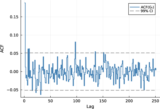
- Can a simple regime-switching model reproduce the three well-known facts of daily stock returns? 1) Big moves happen more often than a normal bell curve predicts (heavy tails), 2) Day-to-day returns don’t “line up” (very low simple autocorrelation), 3) The size of moves tends to stay big or small for a while (volatility clustering).
- Is the old failure of small regime models just because they used the wrong shape for daily returns (normal bell curve), or because they didn’t have enough regimes?
- Can using “heavy-tailed” shapes (that allow more big jumps) fix the problem without adding lots of complexity?
- Can the model give reliable, regime-aware risk forecasts, like Value-at-Risk (how bad a day could be with high confidence)?
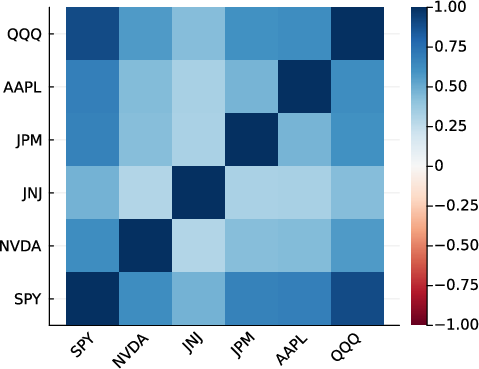
- Can it also handle multiple stocks together, keeping each stock’s behavior while reproducing how they move together?
How did they approach it?
Think of the market as having a few hidden moods. Each day:
- The hidden mood may stay the same or change to another (this is the “Markov chain”: a set of states and transition probabilities).
- Given the current mood, the day’s return is drawn from a distribution that matches that mood’s behavior (its average, variability, and how often extreme moves occur).
Key ideas explained simply:
- Hidden Markov Model (HMM): A model where you don’t directly see the state (mood), but you see signals (returns) produced by that state.
- “Emissions”: The shape of daily returns in each mood. The paper compares four families:
- Gaussian (normal bell curve),
- Student‑t (heavier tails—big moves more likely),
- Laplace (also heavier tails),
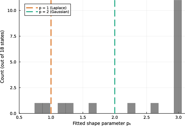
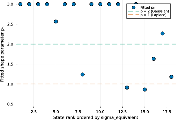
- Generalized Error Distribution (a flexible family that can look like Gaussian or Laplace or in-between).
- Training the model (EM algorithm): A “guess‑and‑improve” loop: 1) E‑step: Given current guesses, estimate the chance each day belonged to each mood (looking forward and backward across the data—like reading a story from both ends). 2) M‑step: Update the model’s parameters (how often moods switch and what each mood’s return shape looks like) to fit those estimates better.
- Smart starting point: They sort returns and split them into chunks to seed initial moods in different parts of the distribution, so the model starts with clearly separate moods.
- Why earlier small models seemed to fail: The authors show mathematically that the “persistence” of volatility (that slow fading of the autocorrelation of absolute returns) is like mixing a few “echoes.” Each echo fades at a certain rate; a few echoes are often enough. The old results likely failed because the daily return shape (Gaussian) was too thin in the tails, not because more echoes (states) were always needed.
- Multi‑asset glue (copula): To simulate several stocks together, they keep each stock’s fitted behavior and use a “copula” (think of it as dependence glue) to arrange the joint moves so correlations look right—without changing each stock’s individual behavior.
Where did they test it?
- A decade of SPY (S&P 500 ETF) with out‑of‑sample testing,
- A panel of 30 large U.S. stocks across 10 sectors,
- A transfer test across different decades,
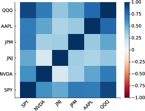
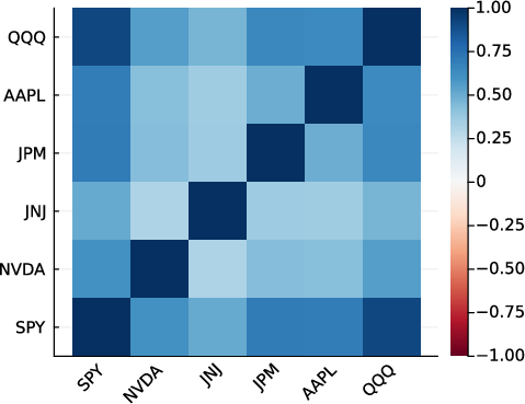
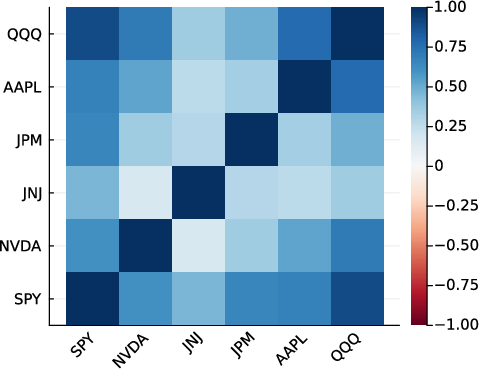
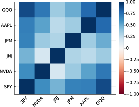
- A 6‑asset basket (e.g., SPY, AAPL, etc.) for multi‑asset behavior.
What did they find, and why does it matter?
- A few moods are enough if the per‑mood return shapes allow heavy tails:
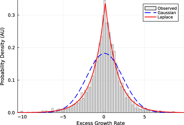
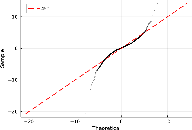
- With 3 states and heavy‑tailed emissions (especially Student‑t), the model reproduced all three “stylized facts” of daily returns: heavy tails, low simple autocorrelation, and long‑lasting volatility clustering.
- Making the return shapes more flexible (heavier tails) helped more than piling on lots of extra states in most cases they studied.
- The “echoes” limit wasn’t the main bottleneck:
- The number of fading modes (echoes) available is limited by the model’s state switching. But on typical U.S. stock data they tested, this limit usually didn’t block a good fit once they had a few states.
- Risk forecasts improved when conditioned on regimes:
- Their regime‑aware Value‑at‑Risk (VaR) passed standard backtests (including a joint conditional coverage test), meaning the model gave realistic estimates of how bad bad days could be, given the current regime.
- Multi‑asset behavior looked more realistic with a Student‑t copula:
- The model preserved each stock’s own shape and used a heavy‑tailed copula to better capture how assets move together, beating a simple single‑factor approach in their tests.
- Baselines:
- A simple “shuffle the past” bootstrap and a semi‑Markov model sometimes matched or beat raw single‑window distribution fit. But they lacked two big advantages of this approach: regime‑aware risk forecasts and a clean way to combine multiple assets while preserving each stock’s behavior.
Why is this important?
For people who test trading strategies, plan for shocks, or build risk controls, you want fake data that looks and “feels” like the real market—not just average days but also rare, large moves and clustered volatility. This paper shows a method that is:
- Interpretable (few regimes with clear meanings),
- Flexible enough to handle heavy tails,
- Good at reproducing key return features,
- Usable for both single‑stock and multi‑stock simulation,
- Able to provide regime‑aware risk forecasts that hold up in backtesting.
Final takeaways and practical notes
- If you want realistic daily stock return simulations, use a few regimes and heavy‑tailed per‑regime distributions (like Student‑t).
- You don’t usually need lots of regimes; better tail shapes often matter more.
- For portfolios, keep each asset’s fitted behavior and add a Student‑t copula to model how they move together.
- This works best for daily U.S. equities in relatively stable periods. Markets change, so you should refit the model periodically.
- The method is meant for creating realistic scenarios, not for ensuring data privacy.
Knowledge Gaps
Knowledge gaps, limitations, and open questions
The paper advances CHMMs with heavy-tailed emissions for daily US equities, but it leaves several concrete issues unresolved that future research could address:
- Emission asymmetry and leverage effects: Only symmetric emission families (Gaussian, Laplace, GED with symmetric shape, Student-t) are used. Evaluate skewed alternatives (e.g., skewed-t, generalized hyperbolic, normal-inverse-Gaussian) and state-dependent asymmetry to capture negative skew and leverage (return–volatility asymmetry).
- Long-memory vs finite geometric modes: The spectral identity shows finite sums of geometric decays; quantify how many modes are needed to approximate empirical power-law decay and benchmark against FIGARCH/HAR/multifractal models. Provide approximation-error diagnostics for the ACF tail.
- Statistical significance of ACF modes: Develop tests with confidence intervals to determine the number and weights of significant eigenvalue modes in Eq. (ACF identity), and assess sampling variability and identifiability of near-unit eigenvalues.
- Squared-return ACF: Extend the spectral analysis and empirical fit to the ACF of squared returns, ensuring the fourth-moment condition holds and reporting how well the model reproduces this target.
- Semi-Markov durations: Although CHMMs performed well, geometric sojourns may still misfit empirical durations. Investigate explicit-duration (HSMM) variants with heavy-tailed emissions that retain regime-conditional VaR and multi-asset composition, and compare complexity–benefit trade-offs.
- Non-stationarity handling: Static transition matrices struggle in stress folds (e.g., COVID, 2022 hikes). Explore time-varying/inhomogeneous HMMs, online EM, change-point detection, regime-split refits, or forgetting factors; quantify gains vs complexity.
- Real-time regime inference: Clarify and enforce use of filtered (not smoothed) state probabilities for live VaR to avoid look-ahead bias; quantify any performance drop relative to smoothed probabilities.
- VaR and ES scope: Backtests focus on 1-day VaR and Kupiec/Christoffersen tests. Add multi-horizon (e.g., 5-, 10-day) VaR, multiple quantiles (1%, 0.5%, 0.1%), and ES backtests (e.g., Acerbi–Szekely), including portfolio-level risk under the copula.
- Parameter uncertainty: The ML-EM framework reports no standard errors or uncertainty quantification. Provide bootstrap/Bayesian intervals for emission and transition parameters, and propagate uncertainty into risk forecasts (predictive distributions).
- EM convergence and local optima: ECM steps (t and GED) use bounded searches without guaranteed monotonicity; quantile-based initialisation may still trap in local maxima. Systematically study multiple restarts, alternative initialisations (k-means/medoids, robust clustering), and convergence diagnostics.
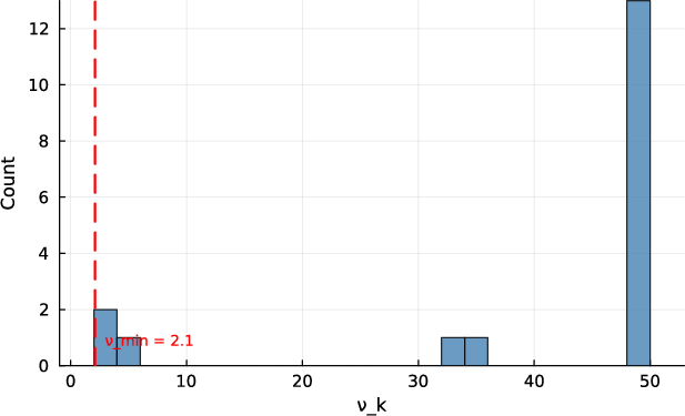
- Hyperparameter bounds and penalties: Degrees-of-freedom (t) and shape (GED) bounds and the t-penalty (λ) strongly affect tails and moments. Report chosen bounds, justify them, and run sensitivity analyses across tickers; ensure required moments exist for ACF targets and risk metrics.
- Model selection for K: Selection by BIC and limited CV showed K=3 ≈ K=6; provide a more general K-selection protocol (e.g., predictive log-likelihood, ICL, marginal likelihood) and investigate label-switching and state redundancy (merging/splitting criteria).
- Rank-bound diagnosis generality: The “rank not active” finding is empirical and variable across tickers. Characterize data features (e.g., state separation, volatility heterogeneity) that predict when the finite-mode bound binds, and provide uncertainty bands for dominant-mode share estimates.
- Copula limitations: The static Student-t copula assumes symmetric, time-invariant dependence and no lead–lag. Test asymmetric/dynamic copulas (Clayton/Gumbel/rotated, time-varying/vine, DCC-copula), evaluate tail-dependence asymmetry, and compare to factor copulas at higher dimensions.
- Preservation of temporal dependence under reordering: Rank reordering preserves marginals and contemporaneous dependence but can distort each asset’s temporal structure and cross-asset co-volatility clustering. Quantify this distortion and explore conditional reordering or copulas applied to innovations/residuals.
- Scaling to higher dimensions: The multi-asset study uses six assets. Assess performance and computation for 50–500 assets (regularized covariance, vine/factor copulas, composite likelihood), and study stability of dependence estimation under heavy tails.
- Joint-regime models across assets: Compare the “independent per-asset CHMM + copula” to coupled/factor HMMs where assets share common latent regimes, and evaluate gains in co-movement, crisis coalescence, and scenario realism.
- Baseline breadth and fair comparison: Main-table baselines omit some strong alternatives (e.g., FIGARCH/HAR, modern diffusion/score-based time-series generators). Include these with proper likelihood or proper-score comparisons and Diebold–Mariano/SAP tests.
- Evaluation under dependence: KS is descriptive with serial dependence. Systematically use dependence-robust metrics (block-bootstrap-calibrated KS/AD, energy distance, MMD with wild bootstrap), report uncertainty on ACF-MAE, and include predictive log-score/CRPS with confidence intervals.
- Scenario simulation from specific regimes: Simulations start from the stationary distribution. Add conditional simulation beginning in filtered stress regimes to support targeted stress testing; quantify differences vs stationary starts.
- Asset-class and frequency generalization: The GLD example failed under static fit. Test adaptive CHMMs on commodities/FX/rates/crypto and higher-frequency (intraday) data with microstructure-aware preprocessing; document required modifications and performance limits.
- Skew and leverage diagnostics: Beyond matching symmetric Cont facts and kurtosis, report skewness targets, return–volatility cross-correlation (leverage), and signed tails; show how enhancements (skewed emissions or regime asymmetry) affect these.
- Dividend adjustments and r_f: Prices are split-adjusted but not dividend-adjusted, and r_f is set to zero. Quantify the impact of dividend and nonzero r_f adjustments on fitted parameters, kurtosis, and risk metrics, especially for dividend-heavy tickers.
- Parameter drift and refit cadence: Provide empirical drift measures of T and emission parameters across walk-forward folds and a data-driven refit cadence heuristic; test robustness of state interpretation across refits.
- Computational scaling and numerics: Detail runtime/complexity vs K, T, and tickers; assess stability of log-space recursions at higher K; explore parallelization/GPU acceleration; document failure modes (state collapse, underflow) and mitigations.
- Privacy: The synthetic series offer no formal privacy guarantees. Explore differential privacy or other privacy-preserving training schemes and quantify utility–privacy trade-offs.
Practical Applications
Practical Applications Derived from the Paper
Below are concrete applications that flow from the paper’s findings, methods (unified EM for CHMMs with heavy-tailed emissions), spectral diagnostics, regime-conditional VaR, and multi-asset copula composition. Each item includes sector linkage, potential tools/workflows, and key assumptions or dependencies.
Immediate Applications
The following can be deployed now with standard risk/quant infrastructure and the paper’s released methodology.
- Regime-conditional daily VaR for equity books (finance: banks, asset managers, hedge funds)
- What: Use the fitted CHMM-t/GED to compute state-probability–weighted (filtered/smoothed) VaR and ES, and backtest with Kupiec/Christoffersen conditional coverage.
- Tools/workflows: “Regime risk” module that ingests daily returns, runs HMM filtering, outputs 1–10 day VaR bands; automated Christoffersen backtest dashboard; alerting when conditional coverage deteriorates.
- Assumptions/dependencies: Daily US equities; reasonably stationary out-of-sample windows; periodic refitting (walk-forward cadence); enough history (≈2,000+ daily points); choose filtered (not smoothed) probabilities in live use to avoid look-ahead.
- Scenario generation for stress testing and backtesting (finance, regtech)
- What: Generate synthetic equity return paths that reproduce heavy tails, negligible linear autocorrelation, and slow decay in |returns| ACF; design stress scenarios absent from observed history.
- Tools/workflows: Synthetic-path API (seeded, reproducible); scenario library tagged by regime mix; batch Monte Carlo for P&L attribution and tail loss envelopes.
- Assumptions/dependencies: Fit CHMM with heavy-tailed emissions (Student-t / GED) and K≈3–6; stationary block bootstrap optional for KS recalibration; no formal privacy guarantees (use caution for data sharing).
- Multi-asset joint simulation via copula composition (finance: portfolio/risk, factor research)
- What: Couple per-asset CHMM marginals with a Student-t copula fitted via Kendall’s τ; simulate joint paths that preserve each asset’s marginal while matching cross-asset dependence.
- Tools/workflows: “Copula composer” that takes single-asset CHMMs, estimates copula (ν, ρ), and generates ranked/reordered paths for portfolios; risk-parity and factor-stress testing.
- Assumptions/dependencies: Assets fitted independently; dependence captured only via the copula (static across the window); Student-t copula suitability; scale-up to >6 assets may require DCC or vine copulas.
- Regime-aware position sizing and volatility targeting (finance: execution/trading)
- What: Map regime probabilities to volatility regimes and adjust target vol/position sizes, stops, and leverage in real time.
- Tools/workflows: Online filtering of γt(k); translation to vol buckets and sizing rules; governance thresholds for regime changes.
- Assumptions/dependencies: Use filtered probabilities; daily cadence; model recalibration when diagnostics degrade.
- Model selection and diagnostics using the spectral rank identity (industry/academia)
- What: Use the “rank of T − 1π̄ᵀ” diagnostic to decide whether to add states (more decay modes) or to increase marginal flexibility (heavier tails) to close fit gaps.
- Tools/workflows: “Spectral dashboard” reporting non-unit eigenvalues, mode contributions, and ACF-MAE; guidance: if dominant mode explains most ACF, prioritize emission family over more states.
- Assumptions/dependencies: Irreducible, aperiodic transition matrix; stationary regime mix in the evaluation window; diagnosis shown effective on typical US-equity tickers.
- Robust, interpretable alternative to deep generators for equity returns (finance, academia)
- What: Use CHMM-t/GED for interpretable generative baselines (states, transitions, per-state parameters) in lieu of opaque deep generators when explainability and reproducibility are required.
- Tools/workflows: Benchmark harness with KS/AD/CRPS/ACF-MAE; seeded generation; parameter snapshots and audit trails.
- Assumptions/dependencies: Focus on daily US equities; periodic refit; ensure state identifiability via quantile-based initialization to avoid degeneracy.
- Data augmentation for ML backtests and strategy research (finance, fintech)
- What: Augment limited equity histories with synthetic samples that preserve stylized facts for robust hyperparameter tuning and stress exposure analysis.
- Tools/workflows: “Synthetic fold” generator for cross-validation; integration into ML pipelines (walk-forward, nested CV); signature-distance/proper-score checks.
- Assumptions/dependencies: Confirm out-of-sample diagnostics; no privacy guarantees (do not use to share confidential data externally).
- Teaching and curriculum modules on stylized facts and HMMs (education, academia)
- What: Course labs demonstrating heavy tails, volatility clustering, state inference, and VaR backtesting using a unified EM framework across emission families.
- Tools/workflows: Ready-to-run notebooks (Julia/Python) for CHMM-N/t/L/GED; spectral ACF identity demos; copula composition exercise.
- Assumptions/dependencies: Use public tickers (e.g., SPY) and provided seeds for reproducibility.
- Vendor productization: CHMM-based risk analytics as a service (fintech, data vendors)
- What: Offer APIs for calibrated CHMM parameters, regime probabilities, VaR/ES, synthetic scenarios, and copula-composed joint simulations.
- Tools/workflows: Scheduled refitting pipeline; SLA around walk-forward diagnostics; client-side plug-ins for OMS/RMS integration.
- Assumptions/dependencies: Transparent documentation of limits (scope: daily US equities; periodic refit); client governance for use in capital calculations.
Long-Term Applications
These require further research, scaling, or development beyond the paper’s scope and validations.
- Online/streaming regime models for non-stationary markets (finance)
- What: Combine CHMM with online EM, change-point detection, or Bayesian updating to adapt regimes in real time.
- Tools/workflows: Drift detectors, sliding-window refits, or BOCPD; automated model selection (states vs. emissions) via live spectral diagnostics.
- Assumptions/dependencies: Robustness to regime drift; latency constraints; careful backtesting to avoid overreaction to transients.
- Higher dimensions and dynamic dependence (finance: multi-asset risk)
- What: Scale from 6 assets to tens/hundreds with DCC, dynamic/vine copulas, or composite-likelihood covariance estimators; allow time-varying copula parameters.
- Tools/workflows: Hybrid: per-asset CHMM marginals + DCC/vine; parallelized simulation; rolling dependence estimation.
- Assumptions/dependencies: Sufficient data for stable high-dimensional dependence estimates; computational scaling; governance for model complexity.
- Intraday/finer-frequency extensions (trading, market microstructure)
- What: Adapt CHMM to intraday bars with microstructure noise handling, irregular sampling, and volatility seasonality; regime-aware intraday risk and sizing.
- Tools/workflows: Preprocessing (de-seasonalization, liquidity filters); multi-frequency calibration; state persistence constraints across sessions.
- Assumptions/dependencies: New preprocessing and state-duration controls; potentially semi-Markov or duration-penalized transitions; expanded validation.
- Duration-aware regimes to approximate long memory (finance, methods)
- What: Integrate hidden semi-Markov (HSMM) durations or hybrid CHMM-HSMM to better match long-memory volatility beyond geometric modes.
- Tools/workflows: Duration-augmented forward-backward; model selection between CHMM and HSMM using ACF/score metrics.
- Assumptions/dependencies: Increased complexity and compute; risk of overfitting; careful out-of-sample validation.
- Derivatives risk and scenario analytics (sell-side/market makers, buy-side overlays)
- What: Combine CHMM returns with option-implied dynamics (e.g., realized–implied bridges) to generate scenarios for Greeks, P&L VaR/ES, and stress impacts.
- Tools/workflows: Joint calibration to returns and implied vols; scenario shocks consistent with smile/skew; copula across underlyings.
- Assumptions/dependencies: Additional models for implied dynamics; reconciliation between physical and risk-neutral measures.
- Policy and supervisory stress testing with standardized synthetic libraries (policy, regtech)
- What: Curate regulator-approved synthetic scenario sets with documented coverage and backtests; supplement scarce stress episodes.
- Tools/workflows: Public scenario repositories; uniform backtesting protocols (Christoffersen/Kupiec/CRPS); model risk disclosures.
- Assumptions/dependencies: Governance for model transparency and limitations; oversight for non-stationarity and structural breaks; caution: no privacy guarantees as-is.
- Privacy-preserving synthetic market data (regtech, data sharing)
- What: Add differential privacy or posterior sampling over parameters to mitigate re-identification risk in shared synthetic datasets.
- Tools/workflows: DP mechanisms at parameter or simulation stage; utility–privacy evaluation; sector-specific release policies.
- Assumptions/dependencies: Trade-offs between fidelity and privacy; rigorous audits; regulatory acceptance.
- Cross-asset class generalization (rates, FX, commodities, crypto)
- What: Extend to assets where heavy tails and clustering differ (e.g., commodities, GLD, crypto), potentially with dynamic fitting or frequency-specific preprocessing.
- Tools/workflows: Asset-class–specific diagnostics; alternative emissions (asymmetric, skew-t), state-duration constraints, or exogenous covariates.
- Assumptions/dependencies: The paper reports a breakdown on GLD under static fitting; requires new validation and potentially different model components.
- Retail risk advisory and robo-advisors (daily life/fintech)
- What: Regime-aware risk indicators for portfolios (e.g., “risk beacon” badges), daily VaR bands, and scenario explainers for non-experts.
- Tools/workflows: Simplified front-ends; plain-language regime summaries; suitability controls; guardrails to prevent procyclical de-risking.
- Assumptions/dependencies: Robustness and explainability; strict compliance and client disclosures; prudent limits on automation.
- Exogenous-driver and macro-linked regimes (academia, macro-risk)
- What: Incorporate macro variables as covariates in transitions or emissions to interpret regime drivers and create macro-conditional scenarios.
- Tools/workflows: Markov-switching with covariates; Granger and causal tests; macro scenario engines linking regime probabilities to narratives.
- Assumptions/dependencies: Risk of overfitting; stability of macro–market links across cycles; transparent model governance.
Notes on general assumptions across applications:
- Scope: daily US equities with stable out-of-sample periods; regime drift requires walk-forward refitting. The finite-state HMM provides a finite set of geometric ACF modes; heavy-tailed emissions were critical to match kurtosis.
- Data needs: sufficient sample length (multi-year daily history), consistent pricing (VWAP or close), and careful vendor joins.
- Validation: rely on multiple metrics (KS/AD/CRPS/ACF-MAE/kurtosis) and conditional coverage for VaR.
- Limitations: finite-state HMM does not imply true long-memory/power-law decay; no formal privacy guarantee for synthetic series; GLD example shows that static fitting can fail outside scope, motivating dynamic or asset-specific extensions.
Glossary
- Absolute growth-rate ACF: The autocorrelation function computed on the absolute values of growth rates, used to quantify volatility clustering. "A standard closed-form identity for the absolute growth-rate ACF, written as a sum over the non-unit eigenvalues of the transition matrix"
- ACF-MAE: Mean absolute error between observed and simulated absolute (and raw) growth-rate ACFs across lags. "ACF-MAE = mean absolute error of the absolute growth-rate / raw growth-rate ACF over $252$ lags."
- Anderson–Darling (AD) test: A goodness-of-fit test emphasizing tail differences between distributions. "Auxiliary distributional metrics (block-bootstrap KS recalibration, Anderson-Darling (AD), Wasserstein-1 (), Hellinger distance, and continuous ranked probability score (CRPS)) are reported in the appendix"
- Aperiodic (Markov chain): A property ensuring a Markov chain does not cycle with a fixed period, helping guarantee a unique stationary distribution. "A unique exists when is irreducible (every state can eventually be reached from every other) and aperiodic (returns to a state are not locked to a fixed period)"
- Baum–Welch algorithm: The EM algorithm specialization for HMMs, providing closed-form updates for Gaussian emissions. "the classical Baum-Welch M-step updates them in closed form"
- Bayesian Information Criterion (BIC): A model selection criterion penalizing complexity to avoid overfitting. "and the Bayesian information criterion (BIC) also picked ."
- Block bootstrap (stationary): A resampling method preserving temporal dependence by resampling blocks of observations. "A stationary block bootstrap at mean block length gave broadly overlapping IS and OoS CIs"
- C-vine (vine copula): A hierarchical copula construction built from pair-copulas; useful for high-dimensional dependence. "and a truncated C-vine are reported in the appendix as multi-asset comparators."
- Centred transition matrix: The transition matrix after subtracting the outer product of the stationary distribution, used in spectral rank diagnostics. "their number bounded by the rank of the centred transition matrix"
- Christoffersen joint conditional-coverage test: A backtest assessing both coverage and independence of VaR exceptions. "The regime-conditional VaR passed the Christoffersen joint conditional-coverage test"
- Continuous Hidden Markov Model (CHMM): An HMM with continuous-valued emissions governed by per-state probability densities. "We answer this with an established model class, the continuous-emission hidden Markov model (CHMM)"
- Continuous Ranked Probability Score (CRPS): A proper scoring rule for probabilistic forecasts comparing predictive CDFs to observations. "Auxiliary distributional metrics ... and continuous ranked probability score (CRPS) are reported"
- Copula: A function linking multivariate distributions to their marginals to model dependence separately from univariate behavior. "Sklar's theorem says any joint distribution factors into its one-asset marginals and a copula"
- Dynamic Conditional Correlation (DCC) model: A time-varying correlation model for multivariate volatility processes. "Dynamic-conditional-correlation models~\cite{engle2002dynamic}"
- ECME (Expectation/Conditional-Maximisation Either): An EM variant maximising the observed-data likelihood in some steps to improve convergence. "the expectation/conditional-maximisation-either (ECME) variant of \citet{liu1995ml}"
- ECM (Expectation Conditional Maximisation): An EM variant performing sequential conditional maximisations over parameter blocks. "We use the expectation conditional maximisation (ECM) construction"
- EM (Expectation–Maximisation): An iterative algorithm for maximum-likelihood estimation with latent variables. "We learn , the per-state parameter vectors , and jointly by expectation-maximisation (EM"
- Expected Shortfall (ES): The tail-risk measure equal to the mean loss beyond a VaR threshold. "an expected-shortfall (ES) envelope (the band of simulated ES across paths)"
- Forward–backward recursion: The dynamic programming algorithm computing HMM state posteriors efficiently. "The collection is computed at every E-step by the standard forward-backward recursion"
- GARCH(1,1): A conditional variance model with one autoregressive and one moving-average term in volatility. "the tested GARCH(1,1) specification had a lower Kolmogorov-Smirnov pass rate than the CHMM variants"
- GED (Generalised Error Distribution): A flexible distribution family controlled by a shape parameter, interpolating between Gaussian and Laplace. "The CHMM-GED variant uses the generalised error distribution, "
- GICS (Global Industry Classification Standard): An industry taxonomy used to group companies by sector. "a sector-balanced 30-ticker panel spanning ten GICS sectors"
- GJR–GARCH: A GARCH variant capturing asymmetric volatility responses to positive and negative shocks. "Glosten-Jagannathan-Runkle GARCH, GJR-GARCH, \citealp{glosten1993relation}"
- Hellinger distance: A distributional divergence measuring similarity between probability distributions. "Auxiliary distributional metrics ... Hellinger distance, and continuous ranked probability score (CRPS)"
- Hidden semi-Markov model (HSMM): A hidden-state model with explicit (non-geometric) state-duration distributions. "a maximum-likelihood hidden semi-Markov model (HSMM) beat the CHMM on raw single-window fit"
- i.i.d. bootstrap: A resampling method drawing with replacement from the empirical distribution assuming independence. "An i.i.d.\ bootstrap and a maximum-likelihood hidden semi-Markov benchmark matched or exceeded the model"
- Irreducible (Markov chain): A property ensuring every state can eventually be reached from any other, guaranteeing ergodicity. "A unique exists when is irreducible (every state can eventually be reached from every other)"
- Jordan expansion: A decomposition using Jordan blocks for non-diagonalisable matrices, yielding polynomial-times-geometric terms. "For a non-diagonalisable transition matrix, the corresponding Jordan expansion contains polynomial-times-geometric terms"
- Kendall’s tau: A rank correlation coefficient often used to infer copula parameters. "with its correlation matrix fixed from Kendall's via "
- Kolmogorov–Smirnov (KS) test: A nonparametric test comparing empirical CDFs; here used as a distributional fidelity score. "The two-sample Kolmogorov-Smirnov (KS) pass rate at significance level "
- Kupiec coverage test: A VaR backtest focusing on the unconditional frequency of exceptions. "The Value-at-Risk panel additionally reports the unconditional Kupiec coverage test"
- Laplace distribution: A double-exponential distribution with heavier tails than Gaussian. "The CHMM-L variant uses Laplace, "
- Marginal mixture: The overall one-period distribution obtained by mixing state-conditional emission densities with stationary weights. "We call the marginal mixture: marginal because it averages over the hidden state ... a mixture because it is a weighted sum of the per-state densities."
- Markov-switching GARCH (MS-GARCH): A GARCH model whose parameters switch according to a latent Markov chain. "Markov-switching GARCH (MS-GARCH)~\cite{haas2004new} as the closest regime-switching comparator."
- Non-unit eigenvalues: The eigenvalues of the transition matrix other than 1, which govern decay modes in the ACF. "a sum over the non-unit eigenvalues of the transition matrix"
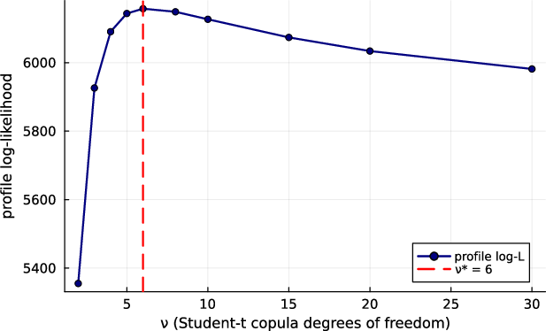
- Profile likelihood: A likelihood function treated as a function of a parameter of interest, maximising over nuisance parameters. "its degrees of freedom are selected by a grid search over the profile likelihood."
- Proper scoring rule: A metric for probabilistic forecasts that is uniquely optimized by the true distribution. "the proper-scoring-rule literature"
- Rank-reordering scheme: A simulation method that imposes a target dependence structure while preserving marginals. "we use the rank-reordering scheme of \citet{iman1982distribution}"
- Regime-conditional Value-at-Risk (VaR): A VaR forecast that conditions on the current estimated regime to capture state-dependent tail risk. "we then build a regime-conditional VaR that forecasts tail risk from the model's running estimate of which regime the day belongs to"
- Rolling-origin cross-validation (CV): A time-series CV method that advances the training window forward before each validation. "under four-fold and six-fold rolling-origin cross-validation (CV"
- Sklar’s theorem: The result that any multivariate distribution can be decomposed into its marginals and a copula. "Sklar's theorem says any joint distribution factors into its one-asset marginals and a copula"
- Sojourn-time distribution: The distribution of durations spent in a state before transitioning, geometric in standard Markov chains. "the geometric sojourn-time distribution of a standard Markov chain"
- Spectral identity: An expression linking ACF decay to the eigen-structure of the transition matrix. "A spectral identity expressed that slow decay as a sum of finitely many geometric modes"
- Stationary distribution: The invariant distribution over states satisfying π̄ = π̄T. "Unconditional simulation initialises the chain from the stationary distribution rather than from the fitted "
- Stochastic volatility: A class of models where volatility follows its own latent stochastic process. "The continuous-latent counterpart is the stochastic-volatility family of \citet{taylor1982financial}"
- Student–t copula: A copula with tail dependence derived from the multivariate Student–t distribution. "We use a Student- copula on the six-asset basket"
- Student–t emissions: Using Student–t distributions as state-conditional emission densities to capture heavy tails. "The CHMM-t variant uses Student-, "
- Stylized facts: Empirical regularities observed across financial time series, such as heavy tails and volatility clustering. "A useful generator should reproduce all of the standard stylized facts of daily returns at once"
- Value-at-Risk (VaR): A quantile-based risk measure indicating a threshold loss not exceeded with specified probability. "Value-at-Risk panel additionally reports the unconditional Kupiec coverage test"
- Wasserstein-1 distance: An optimal-transport metric measuring the cost of moving one distribution to another. "Auxiliary distributional metrics ... Wasserstein-1 () ... are reported"
- Walk-forward (rolling-origin walk-forward): A sequential evaluation method simulating live deployment by refitting and testing as time advances. "a six-fold rolling-origin walk-forward on a decade of SPY"
Collections
Sign up for free to add this paper to one or more collections.