Edge Flow: A Tractable and Predictive Continuous-Time Model for Gradient Descent at the Edge of Stability

Abstract: Gradient descent in deep learning may operate at the edge of stability (EoS), a regime in which the largest eigenvalue of the loss Hessian hovers near the stability threshold $2/η$, where $η$ is the learning rate. Classical analysis tools such as gradient flow and the descent lemma do not apply here, motivating the search for a continuous-time model valid at EoS. We propose Edge Flow, a system of three coupled ordinary differential equations that provides a tractable, faithful, and predictive model of gradient descent dynamics at EoS. Edge Flow decomposes the dynamics into a center, an oscillation direction, and an oscillation magnitude. The center follows a modified gradient flow on a symmetrized loss; the direction tracks a top eigenvector of the Hessian via Rayleigh quotient dynamics; and the magnitude grows or decays exponentially depending on whether the sharpness exceeds or falls below the threshold $2/η$. Crucially, sharpness stabilization emerges from the coupled dynamics via a self-stabilization feedback loop. Discretizing Edge Flow only requires two gradient evaluations and one Hessian--vector product at each iteration. We demonstrate empirically that Edge Flow tracks the dynamics of gradient descent at least as faithfully as previously proposed continuous-time EoS models, while in addition resolving the oscillation of the sharpness at the onset of EoS, and that it provides a principled framework for understanding and mitigating instabilities in this regime.

• The paper introduces Edge Flow, a three-dimensional ODE model that accurately predicts loss spikes and sharpness oscillations at the edge of stability.
• It decouples fast oscillatory behavior from the slow drift of weight centers, linking discretization artifacts directly to observed instability phenomena.
• Empirical validation across architectures like CNNs, ResNets, and ViTs highlights its potential for refining optimization and mitigating training instabilities.

Edge Flow: A Predictive Continuous-Time Model for Gradient Descent Dynamics at the Edge of Stability

Introduction and Motivation

Large learning rates in deep learning often drive gradient-based optimization into the so-called edge of stability (EoS) regime, where the dominant loss Hessian eigenvalue approaches the stability threshold, $2/\eta$, with $\eta$ the learning rate. This phenomenon is pervasive across architectures and training regimes, and is characterized by quasi-periodic oscillations, pronounced loss spikes, and oscillatory sharpness near the threshold. Traditional analytical tools—such as gradient flow and descent lemmas—are inapplicable in this non-smooth, large-stepsize, non-monotonic regime. Existing continuous-time surrogates like Central Flow and Rod Flow either lack tractability or fail to faithfully capture self-stabilization dynamics.

The paper "Edge Flow: A Tractable and Predictive Continuous-Time Model for Gradient Descent at the Edge of Stability" (2606.18080) introduces a three-dimensional ODE system—Edge Flow—that captures the fine-grained and global properties of gradient descent at EoS, elucidates the self-stabilization feedback, and directly connects discretization artifacts to known instability phenomena.

The Edge Flow Model

Edge Flow expresses the GD iterates as oscillating endpoints about a center:

$w_t \approx \bar{w}_t + (-1)^t x_t u_t$

where $\bar{w}_t$ is the slow center, $u_t$ the oscillation direction (unit vector), and $x_t > 0$ the oscillation magnitude. The model decouples the fast oscillatory timescale from the slow drift of $\bar{w}_t$, with dynamical variables governed by the ODE system:

1. Center Dynamics: The center moves according to a gradient flow on a symmetrized potential:

$$\frac{d\bar{w}_t}{dt} = -\frac{1}{2}\left( \nabla L(\bar{w}_t + x_t u_t) + \nabla L(\bar{w}_t - x_t u_t) \right)$$

2. Oscillation Direction: The direction $u_t$ follows the Rayleigh quotient flow to track the dominant Hessian eigenvector:

$$\frac{du_t}{dt} = 2\left( \nabla^2 L(\bar{w}_t) - [u_t^\top \nabla^2 L(\bar{w}_t) u_t]I \right)u_t$$

3. Oscillation Magnitude: The magnitude $\eta$0 evolves exponentially, increasing when the sharpness crosses threshold:

$\eta$1

where $\eta$2.

A key point is that sharpness regulation and loss spikes are emergent properties of these coupled dynamics, rather than imposed constraints, distinguishing Edge Flow from Central Flow and Rod Flow.

The first figure demonstrates Edge Flow’s efficacy in tracking loss and sharpness oscillations, including overshoots at EoS onset, on a ViT trained with MSE loss.

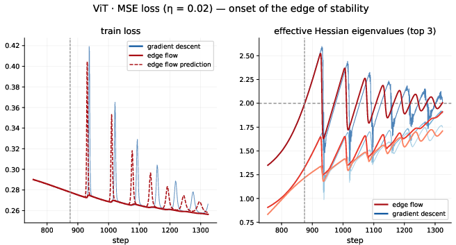
Figure 1: Edge Flow precisely tracks loss spikes and sharpness oscillation at the edge of stability, closely matching gradient descent and capturing features Central and Rod Flow models miss.

Discretization: Edge Gradient Descent

For simulation and practical usage, Edge Flow is discretized as the Edge Gradient Descent (EGD) algorithm. Each EGD iteration requires two gradient evaluations and a single Hessian-vector product—making it computationally competitive (about 3x a GD step with $\eta$3). The step size $\eta$4 is decoupled from training learning rate $\eta$5 and used for numerical integration, enabling fine control over discretization errors. The magnitude update directly encodes the onset of instability at the sharpness threshold, and large $\eta$6 can smooth out transient loss spikes.

Empirically, as shown in further figures, EGD tracks GD oscillations in both center and sharpness in a range of architectures (CNNs, ResNets, ViTs) and loss functions.

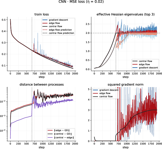
Figure 2: Edge Flow (red) and Central Flow (black) closely track gradient descent (blue) in loss, sharpness, and gradient-norm metrics across CNN training at EoS.

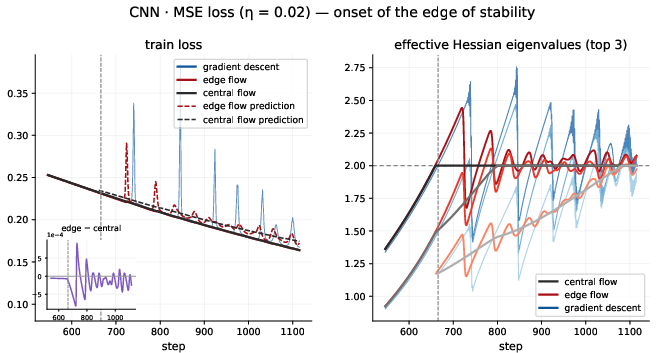
Figure 3: Edge Flow uniquely captures sharpness overshoot and damped oscillation at EoS onset, unlike projection-based Central Flow.

Analysis and Interpretation

The derivation from first principles leverages GD’s two-scale decomposition and symmetry properties at EoS. Notably, the system’s self-stabilization arises from the feedback loop between $\eta$7 (the oscillation) and $\eta$8: growing oscillations steer $\eta$9 toward flatter regions, mechanically adjusting the sharpness to oscillate around its critical value. This negative feedback loop is not enforced but is an emergent result, validated by dynamic tracking of loss spikes and oscillatory sharpness in experiments.

Further, the discretization analysis directly ties the transient loss spikes at EoS onset to numerical stiffness in $w_t \approx \bar{w}_t + (-1)^t x_t u_t$0’s ODE. By refining the center’s discretization or injecting small oscillation base levels ($w_t \approx \bar{w}_t + (-1)^t x_t u_t$1), loss spikes can be controlled or eliminated, as demonstrated in:

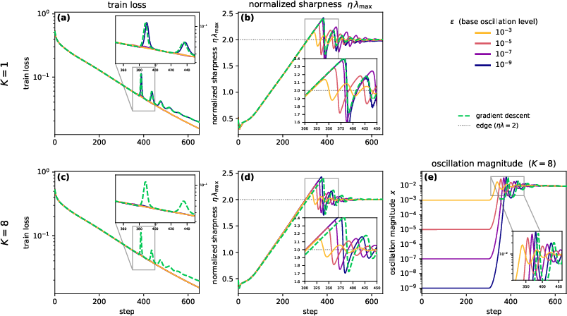
Figure 4: Increasing oscillation base $w_t \approx \bar{w}_t + (-1)^t x_t u_t$2 or integration steps $w_t \approx \bar{w}_t + (-1)^t x_t u_t$3 significantly suppresses loss spikes and sharpness overshoot at EoS onset for MLPs.

Comparison to Alternative Flows

The paper systematically compares Edge Flow to Central Flow and Rod Flow. Central Flow, while capturing the global structure, projects iterates onto the boundary manifold $w_t \approx \bar{w}_t + (-1)^t x_t u_t$4, instantaneously clamping sharpness and missing the physical delay and ringing observed in GD and Edge Flow. Rod Flow, although structurally similar, fails to trigger correct exponential oscillation magnitude growth at the EoS threshold, leading to drift in sharpness beyond $w_t \approx \bar{w}_t + (-1)^t x_t u_t$5.

Edge Flow thus offers the most faithful balance between tractability, fidelity, and predictive power among available continuous-time surrogates.

Implications and Future Directions

Practically, Edge Flow opens avenues for algorithmic refinement of optimization at large learning rates—enabling robust stepsize selection, mitigation of training instabilities, and improved interpretability of implicit regularization phenomena. The explicit modeling of the oscillation center and direction is particularly well-suited for extensions to stochastic methods, adaptive optimizers (e.g., Adam), and architectures with complex curvature spectra.

Theoretically, Edge Flow creates a rigorous framework for analyzing dynamical stability, implicit regularization, and convergence in the non-monotonic, large learning rate regime. Its simplicity lends itself to analytical treatment, possible proofs of self-stabilization feedback, and even making concrete conjectures about the relationship between EoS dynamics, generalization, and margin maximization in deep networks.

The model also suggests algorithmic interventions—such as adaptive integration of the center, artificial noise injection in high-curvature directions, and hybrid methods leveraging both large-step stabilization and fine discretization—which could accelerate training while avoiding loss divergences.

Conclusion

Edge Flow provides a tractable, predictive, and empirically validated continuous-time model for gradient descent at the edge of stability. By decomposing the dynamics into three interpretable components, it not only accounts for oscillatory and instability phenomena observed in deep learning training, but also enables practical algorithmic and analytical advances. Its framework lays a foundation for future exploration of both stable large-stepsize learning and the deeper mathematical structure of high-dimensional nonconvex optimization at criticality.

---

Reference:

"Edge Flow: A Tractable and Predictive Continuous-Time Model for Gradient Descent at the Edge of Stability" (2606.18080)