Blended Chart Surfaces: A Seamless Explicit Representation for Smooth Surface Fitting

Abstract: A surface representation suitable for geometry processing should be compact and explicit, provide global smoothness guarantees, support a wide range of surface topologies, and offer reliable access to differential quantities such as normals and surface energies, while remaining compatible with modern differentiable optimization. Existing neural representations typically sacrifice one or more of these properties: implicit fields typically require iso-surfacing for downstream use, while explicit neural maps are constrained by canonical-domain parametrizations or exhibit seam artifacts between local charts. We introduce Blended Chart Surfaces, a compact, network-free, explicit representation that is smooth by construction and anchored to user-provided topology. Given a coarse proxy mesh encoding the intended surface topology and approximate geometry, Blended Chart Surfaces jointly optimize for a polynomial map at each proxy vertex using an off-the-shelf optimizer to fit to an implicit target shape, avoiding the need for an input parametrization. Neighboring maps are fused using a smooth 'one-ring coordinate' blending scheme, decoupling topology and coarse geometry (carried by the proxy) from geometric details (carried by the local patches). The surface is globally smooth, fully differentiable, and enables stable evaluation of derivatives, making differential quantities and surface energies directly accessible. Additionally, our construction is equivariant to rigid motions and scaling of the proxy mesh. We evaluate Blended Chart Surfaces on various topologies and geometric complexity, and compare against explicit alternatives including interpolating-function baselines and mesh-displacement MLPs. Across these, Blended Chart Surfaces achieve a favorable trade-off among compactness, simplicity, access to differential quantities, and expressivity while remaining smooth across patch boundaries.

• The paper introduces Blended Chart Surfaces (BCS), which uses one-ring local polynomial maps to construct globally C∞ smooth surfaces with explicit differential properties.
• It employs a partition-of-unity blending function to seamlessly merge local patches, resulting in superior reconstruction accuracy and avoidance of artifact-prone discretization.
• Results demonstrate that BCS effectively handles arbitrary topologies and boundaries, making it highly applicable for geometry processing and simulation tasks.

Blended Chart Surfaces: An Explicit, Network-Free, Globally Smooth Surface Representation

Introduction and Motivation

This work presents Blended Chart Surfaces (BCS), an explicit surface representation formulated for geometry processing tasks that require compactness, explicit access to differential quantities (normals, energies), and compatibility with differentiable optimization. Unlike implicit neural representations, which often entail non-differentiable iso-surfacing steps and introduce artifacts during discretization (see Figure 1), BCS constructs a globally $C^\infty$ smooth surface directly over a coarse, user-specified proxy mesh by optimizing local polynomial maps at mesh vertices and blending them using partition-of-unity weight functions.

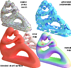
Figure 2: BCS is a compact, network-free, explicit surface representation formed by composing local polynomial maps per proxy vertex, yielding a fully differentiable model faithful to geometry.

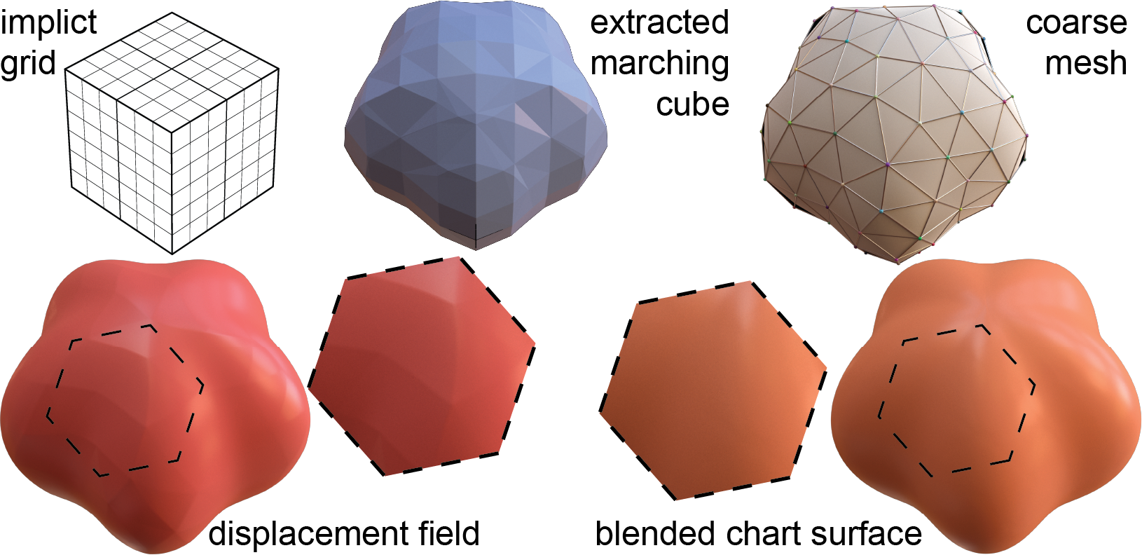
Figure 1: BCS, unlike implicit fields or mesh-based MLP displacements, yields explicit $C^\infty$ smooth surfaces directly from coarse proxies, avoiding artifacts at boundaries.

The formulation achieves equivariance to rigid and scaling transformations, supports arbitrary topology (including non-orientable surfaces and boundaries), and is network-free, facilitating both practical interpretability and theoretical tractability. The crucial innovation is a one-ring coordinate system that allows each vertex's patch to be seamlessly blended with its neighbors, guaranteeing global smoothness across the entire surface (see Figure 3).

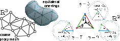
Figure 3: One-ring coordinates are constructed by isometrically flattening the neighborhoods of each vertex and rescaling angles, supporting canonical transition maps for blending.

Method

Local Polynomial Patch Construction and Blending

Given a proxy mesh (triangle soup or polygonal curve), BCS assigns a local map—typically a low-degree polynomial (e.g., quadratic or cubic)—to each vertex. Each map expresses fine geometric details in a frame-aligned, scaled coordinate system anchored at the vertex. These maps are not required to interpolate proxy vertices or the one-ring; instead, their parameters are globally optimized to minimize reconstruction error over a defined target (usually an implicit SDF/gradient).

To blend local maps and enforce smoothness, BCS uses a novel partition-of-unity blending function. For curves (1D case), map supports are overlapping intervals and the blending is done with smooth transition functions satisfying $C^\infty$ continuity and partitioned unity. For surfaces (2D), domains are flattened one-rings, and blending weights are constructed to be $C^\infty$ “hat” functions, determined by radial distance, and normalized across the face (see Figure 4). The overlap region is controlled by a tunable parameter, ensuring per-patch blending is nonzero only within a finite support (see Figure 5, not shown).

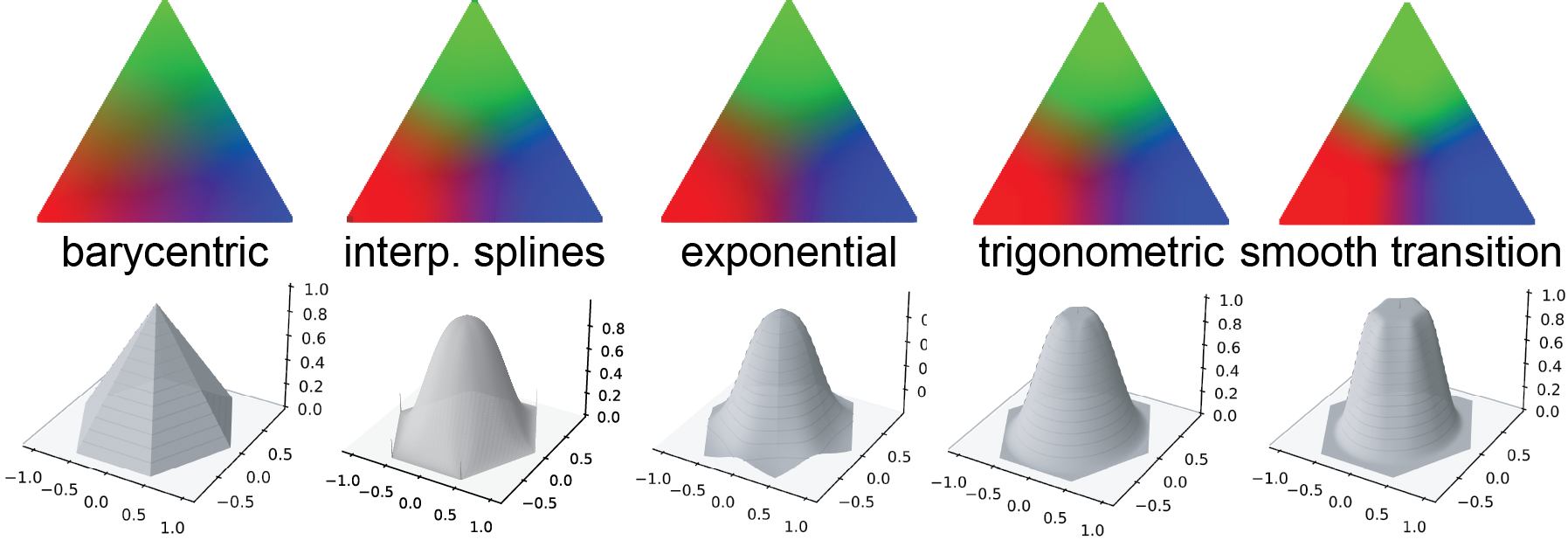
Figure 4: Figure displays blending function alternatives and their induced vertex-centered hat functions, impacting smoothness and locality.

Transition Maps, Equivariance, and Global Smoothness

Transition maps between overlapping local charts are defined by rescaling and angle adjustments to preserve the local neighborhood's combinatorial structure under flattening. This enables blending across arbitrary mesh topologies, including high-valence vertices and non-orientable configurations (Figure 6).

By constructing each vertex function as $p_i(t) = s_i R_i m_i(t) + v_i$ with scale $s_i$, rotation $R_i$, polynomial $m_i$ in local coordinates, and base position $v_i$, BCS inherits equivariance to all affine transformations of the proxy. Partition-of-unity properties in the blending function guarantee translation equivariance, an essential property for geometry processing.

Optimization Objective

The final surface is obtained by optimizing polynomial coefficients to minimize a differentiable loss over the target surface, typically:

• Vertex- or face-wise integrals of SDF values to fit the zero level set,
• Optionally, regularization penalties for normal alignment and area/distance distortion;
• For surfaces with boundaries, an additional term ensures the explicit boundary curve matches the target (see Figure 6).

Thanks to the explicit parameterization, all derivatives and differential quantities (e.g., normals, mean curvature, elastic energy) are available in closed form or via automatic differentiation (see Figures 10 and 11).

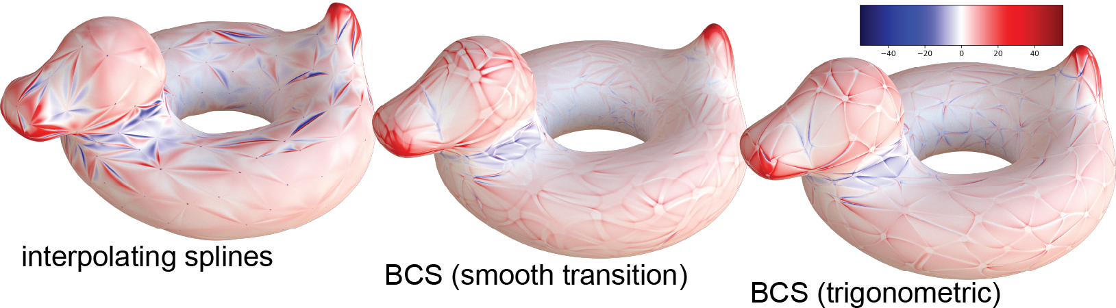
Figure 7: Mean curvature colormaps computed using automatic differentiation demonstrate stable, continuous access to curvature across the BCS surface.

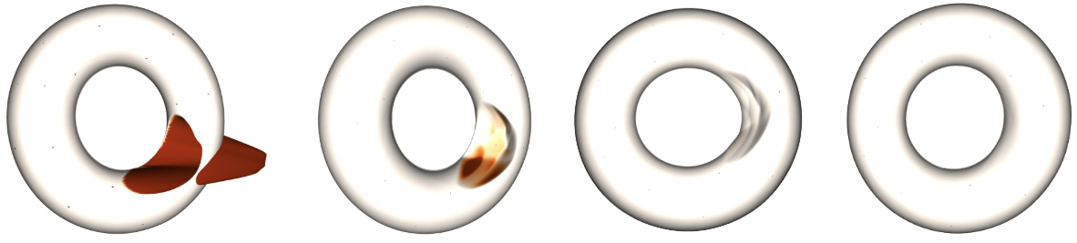
Figure 8: Elastic energy density visualized on a deformed BCS torus, showcasing differentiable simulation—BCS is reoptimized to relax elastic energy.

Handling Arbitrary Topology and Boundaries

BCS naturally handles complex topologies, including genus-$g$ and non-orientable surfaces, since only the proxy mesh's combinatorics are relevant. Non-orientability is handled automatically, as continuity is a local property: angles and normal flips are visualized in Figure 6 but have no impact on smooth blending.

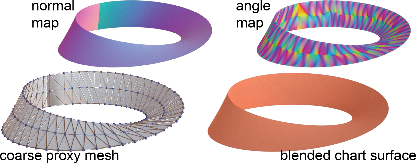
Figure 6: BCS reconstructs a Möbius strip from a coarse proxy mesh, validating natural support for boundaries and non-orientability via local blending.

Results

Surface Quality and Compactness

BCS achieves strong reconstruction accuracy across diverse targets, including both analytic and neural implicit fields (e.g., Igea, Bob, Fertility, and twisted torus), with mean error visualized via heatmaps. Notably, quadratic polynomial patches (i.e., $C^\infty$0 coefficients per vertex) suffice for high fidelity, and smooth transition blending yields visually and quantitatively superior fits compared to mesh-displacement MLPs or classical interpolating splines (Figure 9, Figure 10).

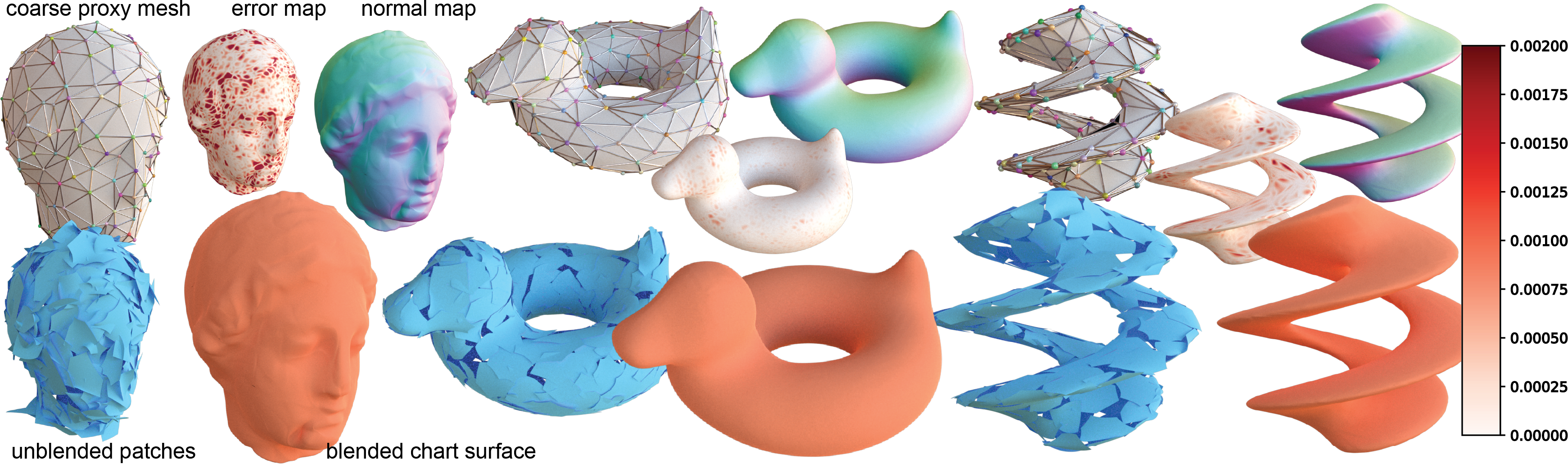
Figure 9: Gallery shows BCS results on three targets, with proxies, unblended patches, blended surfaces, and error maps. Quadratic patches and moderate vertex count suffice for detail and smoothness.

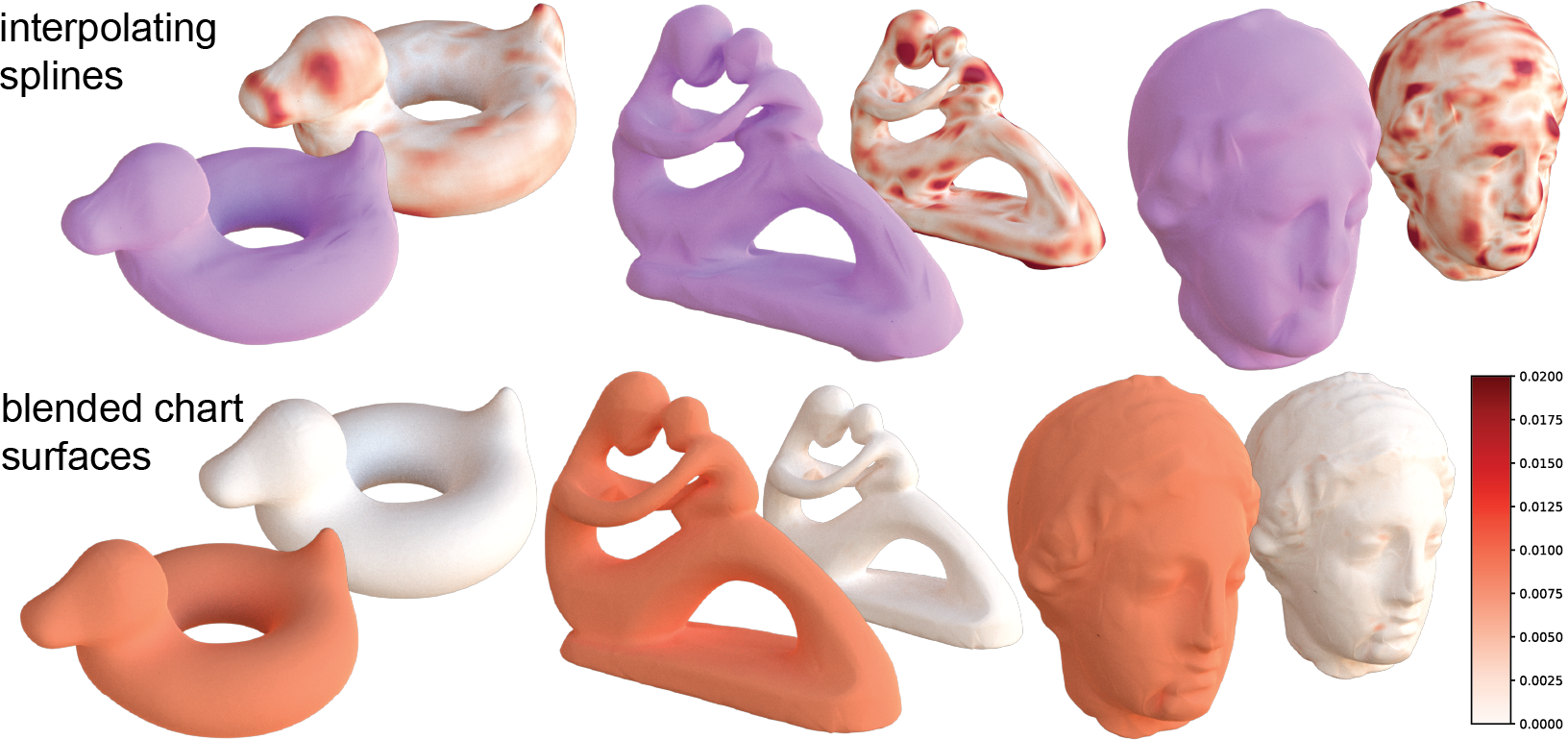
Figure 10: BCS (right) versus interpolating splines of Djuren et al.—joint optimization using the target field leads to superior fits and lower error.

BCS supports a hierarchy of detail: higher polynomial degrees enable finer approximation, while lower degrees yield greater compactness (Figure 11). Increasing proxy mesh resolution improves fitting in regions of high curvature or detail (Figure 12).

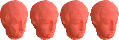
Figure 11: BCS with degree-0 (constant), degree-1 (linear), degree-2 (quadratic), and degree-3 (cubic) polynomials on Igea illustrate progressive improvement in local accuracy.

Differential Geometry and Simulation

BCS surfaces admit robust computation of normals, mean/gaussian curvature, and elastic energies everywhere on the surface, facilitating applications in simulation and physics-based optimization—not common in neural implicit representations (Figure 7, Figure 8).

Blending Function Ablation and Seam Artifacts

Experiments with various blending functions reveal that the choice of blending strategy dramatically impacts surface continuity—barycentric and exponential weighting induce artifacts or holes, while the proposed smooth transition function achieves global $C^\infty$1 smoothness (Figure 13).

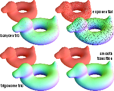
Figure 13: Blending function impacts: barycentric and exponential introduce visible seams and holes, trigonometric blending achieves $C^\infty$2, and smooth transition achieves $C^\infty$3 continuity.

Boundary and Non-Orientable Support

BCS accommodates arbitrary boundary handling by adjusting one-ring flattening for boundary vertices and incorporating additional losses for explicit boundary fits (Figure 6).

Implications and Future Directions

The BCS construction enables practical deployment of explicit, $C^\infty$4 smooth, network-free surfaces that are compact, local, and friendly to differentiable optimization. Numerical and qualitative results indicate that BCS yields significantly improved fidelity—especially across patch/chart boundaries—compared to both traditional mesh-based and deep learning-driven baselines.

Practically, this impacts modeling, simulation, and downstream learning systems that require explicit geometry with stable access to surface properties. Theoretically, BCS provides a template for hybrid representations anchored in classical geometry but compatible with modern optimization. Supporting arbitrary topology and boundaries without seam artifacts removes a central limitation of most explicit neural surface models.

Future direction could explore:

• Feature-aware BCS for piecewise-smooth surfaces with controlled sharpness,
• Generative modeling pipelines (e.g., by regressing polynomial coefficients from latent codes or VLM context),
• Time-varying extensions for animated surfaces,
• Mixed polynomial/spherical/specialized vertex map choices per local area,
• Combining BCS with data-driven proxies.

Conclusion

Blended Chart Surfaces provide an explicit, compact, and globally smooth surface representation leveraging polynomial vertex-centric patches and partition-of-unity blending over a user-specified proxy. The method ensures $C^\infty$5 continuity, local control, equivariance, and direct access to all differential properties, outperforming alternative representations on surface fitting and smoothness metrics. While limitations exist for very coarse proxies or extremely high-curvature features, BCS marks a substantial advance in explicit geometry processing. Extensions to generative, temporal, or mixed topology settings beckon, establishing BCS as a versatile tool for both theoretical and applied research in surface modeling and analysis.

---

This essay summarizes "Blended Chart Surfaces: A Seamless Explicit Representation for Smooth Surface Fitting" (2606.18069).