Neural Legendre-Fenchel transform with Hessian Preconditioning
Abstract: The Legendre-Fenchel (LF) transform is a fundamental tool in convex analysis and machine learning that maps lower semi-continuous functions to their convex conjugates. In practice, when closed-form formula are not available for expressing convex conjugates of given functions, one must approximate them using various techniques. One recent such versatile numerical method is the deep Legendre transform method which relies on neural networks although it remains challenging particularly for tackling ill-conditioned functions. This work builds on the reformulation of the LF transform as a projective polarity. A notable property of this framework is its affine invariance. We leverage this affine invariance to introduce a Hessian-based preconditioning strategy. Specifically, we apply an affine deformation around a minimizer so that the second-order Taylor approximation of the function coincides with the canonical paraboloid, whose conjugation map is the identity. A residual network initialized near the identity can then learn this simplified mapping, while the original conjugation map is recovered through the inverse deformation. The proposed preconditioning incurs only a modest computational overhead, consisting of a single eigendecomposition during initialization and two matrix-vector multiplications per query. Experiments on a diverse set of convex functions, including high-dimensional benchmarks, demonstrate improved convergence rates and enhanced numerical accuracy of the conjugation, with particularly significant gains for ill-conditioned problems. Finally, we discuss the scope of applicability of our proposed method and highlight several of its limitations.
Paper Prompts
Sign up for free to create and run prompts on this paper using GPT-5.
Top Community Prompts
Explain it Like I'm 14
Plain-English Summary of “Neural Legendre–Fenchel Transform with Hessian Preconditioning”
What is this paper about?
This paper is about a math tool called the Legendre–Fenchel transform (LF transform). It turns one “nice, bowl-shaped” function into another related function called its convex conjugate. This tool shows up in physics, optimization, and machine learning (for example, in optimal transport). Sometimes the LF transform is hard to compute exactly, so the authors use a neural network to learn it. Their main idea is a clever “preconditioning” step that reshapes the problem to make learning faster and more accurate.
1) Main Topic and Purpose
The paper introduces a way to make a neural network learn the LF transform more easily and reliably. The trick is to “precondition” (re-scale and re-center) the original function using information about how curved it is near its minimum. This makes the learning task much simpler, so the network trains faster and gives better results.
2) Key Questions the Paper Tries to Answer
- How can we train a neural network to compute the LF transform (or its mapping) when there is no simple formula?
- Can we make this training more stable and faster, especially for tough cases where the function is “ill-conditioned” (stretched a lot in some directions)?
- What simple changes to the input (an affine transformation: shift + stretch/squash) make the LF transform easier to learn without changing the core problem?
3) How the Method Works (in Everyday Language)
Before the steps, here are the main ideas in simple terms:
- Convex function: Think of a smooth bowl. If you roll a marble in it, it ends up at the lowest point.
- Gradient: The slope or direction that points downhill or uphill.
- Hessian: A matrix that measures the bowl’s curvature in every direction (how steeply it curves). A round bowl has the same curvature in all directions; an oval bowl bends more in some directions than others.
- Ill-conditioned: The bowl is very stretched in some directions. That makes learning harder, because small changes along some directions matter much more than others.
- Preconditioning: We change coordinates to make the bowl look more round (like turning an oval bowl into a nearly circular one). This makes the problem much easier.
What they actually do:
- They look near the function’s minimum (the bottom of the bowl) and compute the Hessian there (the “curvature matrix”).
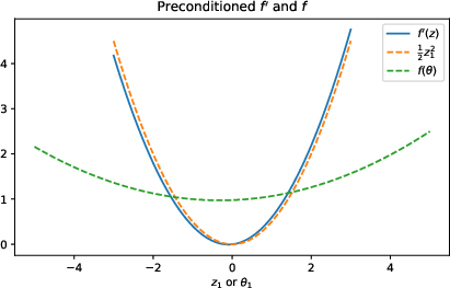
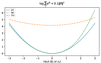
- Using the Hessian, they apply a special affine transformation (a shift and a stretch/squash) so that, near the bottom, the function looks like a perfect paraboloid: Q(θ) = ½||θ||². This “canonical paraboloid” is special because it is its own LF transform and the best mapping is just the identity (input equals output).
- They train a residual neural network that starts very close to the identity mapping. Because the transformed problem is now “almost identity,” the network has an easy job: small corrections instead of learning a complicated map from scratch.
- After the network learns in the transformed space, they “undo” the transformation to get the answer for the original function.
Training objective (what the network minimizes):
- They use a standard convex-analysis loss called the Fenchel–Young loss. You can think of it as a score that measures how well the network’s output matches the true LF transform relationship. Lower is better.
Why this is valid:
- There’s a math result (affine invariance) that says if you stretch/shift the original function in a certain way, the LF transform stretches/shifts accordingly. So, solving the transformed problem and then transforming back gives the right answer for the original problem.
Computing cost:
- One-time cost at the start: find the function’s minimum and compute the Hessian’s eigendecomposition (this tells you how to stretch/squash).
- Tiny extra cost at inference (prediction) time: just two matrix–vector multiplications to transform in and out. That’s fast.
4) Main Findings and Why They Matter
What they tested:
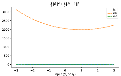
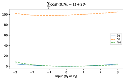
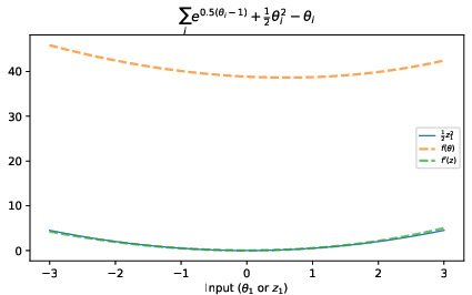
- They tried their method on different kinds of convex functions (quadratics, mixtures with quartic terms, sums of cosh functions, exponentials plus quadratics, and log-sum-exp with regularization).
- They tested across a range of dimensions (from small to higher-dimensional problems).
What they found:
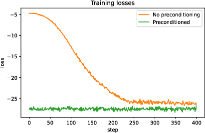
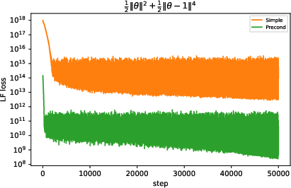
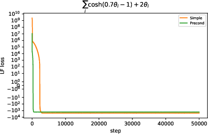
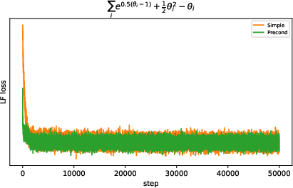
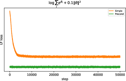
- The preconditioning consistently made training faster and more stable.
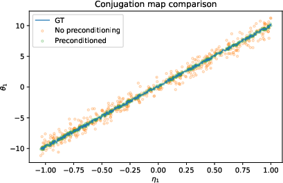
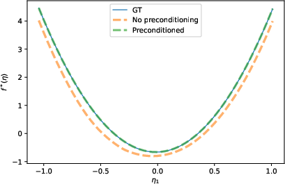
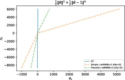
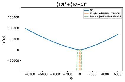
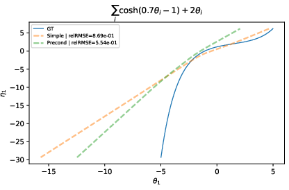
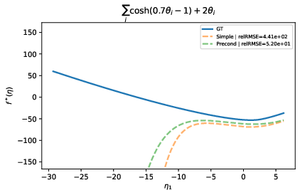
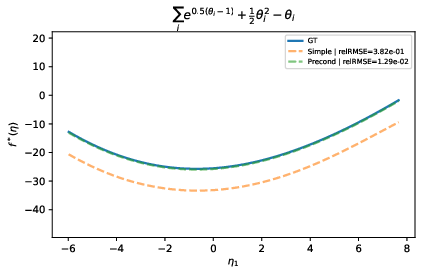
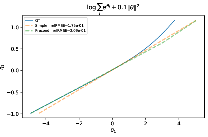
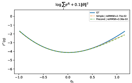
- Accuracy improved, especially for “ill-conditioned” problems (the very stretched bowls).
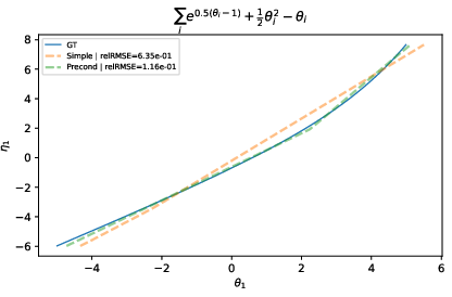
- In many cases, the network learned the correct mapping in far fewer steps and produced more accurate conjugate values.
Why this is important:
- Computing LF transforms shows up as a subroutine in bigger tasks (like optimal transport). Faster, more reliable learning means these larger systems can be more practical and scale better.
- The method adds only a tiny overhead at prediction time, making it attractive in real applications.
5) Implications, Impact, and Limitations
What this could change:
- Makes neural methods for convex conjugation more robust, especially on tough, high-curvature-imbalance problems.
- Could improve tools in machine learning that rely on LF transforms, such as certain optimal transport solvers.
Where it might struggle:
- It needs a real, finite minimum for the function. If the function doesn’t have a true minimum (or it’s extremely hard to find), the setup fails.
- The preconditioning is based on local curvature near the minimum. If the function’s curvature changes a lot far away, the benefits may fade there.
- If the Hessian is nearly singular (some near-zero curvature directions), the stretching step can be unstable; they clamp tiny values, which helps but reduces accuracy.
- If the function is already well-conditioned (already close to a round bowl), preconditioning doesn’t help and just adds small overhead.
- Computing the Hessian can be expensive in very high dimensions; approximations may be needed.
Big picture:
- The paper shows that a smart, math-guided re-shaping of the problem can make neural learning of LF transforms much easier.
- It blends theory (affine invariance and “polarity” geometry) with practical engineering (residual nets, simple initialization, tiny inference overhead), leading to faster and more accurate results in many cases.
Knowledge Gaps
Knowledge gaps, limitations, and open questions
Below is a single, consolidated list of what remains missing, uncertain, or unexplored in the paper. Each point is phrased to be concrete and actionable for future research.
- Lack of formal convergence guarantees: No theoretical bounds are provided on training error or iteration complexity with and without Hessian preconditioning (e.g., dependence on condition number, curvature mismatch, or network capacity).
- Accuracy guarantees for the learned conjugation map: The paper does not derive error bounds for or as a function of distance from the minimizer, Hessian approximation error, or sampling distribution over .
- Applicability beyond Legendre-type functions: The method assumes closed, strictly convex (Legendre-type) functions; its behavior for non-smooth convex functions, extended-real valued functions, or functions with non-invertible gradients is not studied.
- Domain constraints are ignored: The approach is designed for unconstrained ; how to handle convex functions defined over constrained domains (e.g., polyhedral sets, simplices) and their conjugates remains open.
- Multiple minimizers and non-strict convexity: The algorithm hinges on a unique minimizer and a well-defined Hessian at that point; treatment of functions with flat minima, multiple minima, or ill-defined second-order structure is not addressed.
- Preconditioning locality vs. global performance: The benefit is local around ; there is no analysis or method to ensure good conjugation accuracy for queries far from the minimizer, or when curvature varies dramatically across the domain.
- Adaptive or multi-point preconditioning is unstudied: No mechanism is provided to update or the preconditioning on-the-fly, combine multiple local preconditioners, or partition the domain into regions with tailored deformations.
- Robustness to near-singular Hessians is only heuristic: The paper clamps tiny eigenvalues but does not quantify stability thresholds, the effect of regularization on accuracy, or principled alternatives (e.g., ridge regularization, trust-region preconditioning).
- Large-scale Hessian estimation: Computing the full Hessian (or eigendecomposition) is expensive for large ; the effectiveness of approximate Hessians (diagonal, block-diagonal, low-rank, Lanczos/HVP-based) and their trade-offs are not evaluated.
- Choice of affine deformation is ad hoc: Although the polarity framework supports arbitrary affine deformations, there are no criteria or algorithms to learn or select beyond the local Hessian, nor comparisons of different deformations tailored to known structure (e.g., separability, spectra).
- Sampling strategy for training is unclear: The uniform sampling of within a range derived from is not justified; the impact of the sampling distribution on training stability, coverage, and accuracy is unstudied.
- Ground-truth conjugation quality is not validated: The “ground truth” is obtained by inner Adam optimization; there is no quantification of its residual error, sensitivity to optimization settings, or comparison with closed-form conjugates where available.
- Head-to-head benchmarks are limited: There is no direct, standardized comparison against ICNN-based methods, Deep Legendre Transform (DLT), or other amortized conjugation approaches on shared datasets/tasks (e.g., Wasserstein-2 OT benchmarks).
- Lack of evaluation on real-world targets: The method is not tested on the motivating tasks (e.g., log-partition functions of discrete exponential families, practical OT pipelines, real data distributions) where is expensive or only indirectly accessible.
- Dependence on access to function values: Inference of still requires evaluating at the predicted ; scenarios where only or unbiased stochastic estimates of are available are not addressed.
- Training instabilities and overflow: Failures (e.g., quartic mix) due to loss explosion are reported, but strategies to prevent blow-up (normalization, loss scaling, robust objectives, gradient clipping schemes, input standardization) are not systematically developed or evaluated.
- Scalability beyond moderate dimensions: Experiments are limited to ; the computational and statistical scaling of the method (including Hessian cost, training time, and approximation error) for remains uncertain.
- Architecture and initialization choices: The reliance on residual networks initialized near identity is plausible but untested against alternatives (e.g., monotone networks, normalizing flows, spline maps); the sensitivity to depth/width and activation functions is not analyzed.
- Effect of preconditioning on the loss landscape: The claim that the method starts in an “excellent basin” lacks quantitative characterization of the loss geometry pre-/post-deformation (e.g., smoothness, Lipschitz constants, gradient variance).
- Uncertainty quantification is missing: There is no assessment of prediction uncertainty for or (e.g., calibration, confidence intervals, ensemble methods), which would be critical for downstream optimization or OT tasks.
- Out-of-distribution query behavior: The model’s robustness when queried with outside the training range (or far from regions where preconditioning is valid) is not evaluated; no safeguards for extrapolation errors are proposed.
- Impact of clamped eigenvalues on conjugation bias: The trade-off between numerical stability (clamping small eigenvalues) and induced bias in the deformation/conjugation map is not quantified.
- Jointly learning the deformation is untested: While proposed as future work, there is no demonstration of learning jointly with the conjugation network, nor exploration of parameterizations (e.g., SPD factorizations, low-rank updates) or regularization to keep well-conditioned.
- Extensions to stochastic or set-valued settings are speculative: The paper mentions entropic OT and set-valued conjugation maps but does not provide formulations, losses, or experiments for noisy , stochastic conjugates, or multivalued mappings.
Practical Applications
Immediate Applications
Below are concrete use cases that can be deployed now, leveraging the paper’s Hessian-preconditioned neural Legendre–Fenchel (LF) transform to accelerate and stabilize conjugation and conjugation-map learning, especially for ill-conditioned convex functions.
- Sector: Machine Learning (Optimal Transport, Generative Modeling)
- Application: Drop-in preconditioner for neural OT solvers (W2)
- What it enables: Faster, more accurate training of dual potentials and conjugation maps in neural OT pipelines (e.g., W2 generative models, color/shape transfer, domain alignment).
- Tools/workflow: Wrap existing OT code (ICNN-based or amortized approaches) with the preconditioning step: find minimizer θ0, compute Hessian at θ0, transform to z-space, train residual net initialized near identity, invert affine map at inference.
- Assumptions/dependencies: f must be of Legendre type with a finite minimizer; need Hessian (or a stable approximation); largest gains when the problem is ill-conditioned.
- Sector: Machine Learning (Deep Legendre Transform, Amortized Conjugation)
- Application: Speedup for Deep Legendre Transform (DLT)-style methods and amortized conjugation networks
- What it enables: Lower training steps and improved numerical accuracy for learning f* and the map η ↦ θ*(η), without needing ∇f at inference.
- Tools/workflow: Integrate a PyTorch/JAX preconditioning module (single eigendecomposition at setup, two matrix–vector multiplies at inference).
- Assumptions/dependencies: Requires access to f (forward eval), a good θ0 solver, and a numerically stable Hessian.
- Sector: Machine Learning (Fenchel–Young losses, Structured Prediction)
- Application: Faster computation of FY losses via amortized conjugates
- What it enables: Efficient inference for FY-based models (e.g., structured prediction, sparse/entropic regularization) by amortizing θ*(η), reducing per-batch inner optimization.
- Tools/workflow: Train a preconditioned residual net for η ↦ θ(η); compute f(η) ≈ θ·η − f(θ) on-the-fly.
- Assumptions/dependencies: FY loss must be associated with a convex f having a well-defined minimizer and sufficiently smooth curvature near θ0.
- Sector: Data Science and Statistics (Exponential Families, Cumulant/Log-Partition)
- Application: Surrogate conjugates for difficult log-partition functions
- What it enables: Practical approximations of dual mappings and conjugate values for discrete or high-dimensional exponential families where closed forms are unavailable.
- Tools/workflow: Use preconditioned training to learn η ↦ θ(η) using samples from ∇f(θ) if available, or by stochastic approximation of f; reconstruct f when needed.
- Assumptions/dependencies: May require approximate Hessians (diagonal/low-rank) and careful numerical stabilization; gains depend on availability/quality of f and curvature estimates.
- Sector: Optimization/Operations Research (Primal–Dual Methods)
- Application: Acceleration of inner conjugation steps in primal–dual algorithms
- What it enables: Faster iterations in resource allocation, ad auctions, and large-scale convex programs with custom regularizers by amortizing conjugation instead of solving per-iteration argmaxes.
- Tools/workflow: Train once per problem family to learn η ↦ θ*(η); call the amortized map inside a primal–dual loop.
- Assumptions/dependencies: Stable Hessian at a representative minimizer; performance may degrade if the algorithm explores regions far from the preconditioned local geometry.
- Sector: Finance (Risk Measures and Regularization)
- Application: Amortized duals for convex risk regularizers (e.g., CVaR-like or custom penalties)
- What it enables: Speedup of scenario-based optimization and portfolio allocation pipelines that rely on dual representations of convex risk measures.
- Tools/workflow: Train preconditioned conjugation models for the specific regularizer; reuse across runs with varying η.
- Assumptions/dependencies: Need a well-defined minimizer and tractable Hessian or a regularized approximation; deploy with error checks where model risk matters.
- Sector: Scientific Computing/Physics (Hamiltonian–Lagrangian Duality)
- Application: Learned Legendre maps between velocities and momenta
- What it enables: Surrogate inference for Legendre transforms in learned Lagrangians (near equilibrium), enabling fast bidirectional mapping in simulation loops.
- Tools/workflow: Identify local equilibrium θ0, compute Hessian, precondition and train; use the amortized map in integrators or PINN-style frameworks.
- Assumptions/dependencies: Valid near equilibria (locality); strong curvature variation away from θ0 reduces gains.
- Sector: Healthcare and Bioinformatics (OT-based Alignment)
- Application: Faster W2 OT-based data alignment (e.g., single-cell atlas integration, cohort matching)
- What it enables: Reduced compute time and improved stability for high-dimensional, convex-potential-based alignment tasks.
- Tools/workflow: Plug preconditioning into OT solvers within analysis pipelines (e.g., Scanpy/Seurat extensions with OT).
- Assumptions/dependencies: High-dimensional Hessian estimation may require low-rank approximations; ensure compliance with data governance/privacy when estimating f.
- Sector: Software Tooling and Education
- Application: Reusable preconditioning component and didactic demos
- What it enables: A lightweight library/module (e.g., “neural_conjugate_precond”) for PyTorch/JAX that demonstrates polarity-based affine invariance and LF preconditioning; useful for teaching convex duality and modern numerical conjugation.
- Tools/workflow: Provide API for setup (θ0, Hessian), training loop wrappers, and inference utilities.
- Assumptions/dependencies: Basic autodiff backend, eigendecomposition routine, and convexity checks.
Long-Term Applications
Below are forward-looking applications that require further research, scaling, or integration work (e.g., adaptive preconditioning, theoretical guarantees, very high-dimensional deployment).
- Sector: Machine Learning (Adaptive/Online Systems)
- Application: Adaptive or patch-wise preconditioning across input space
- What it enables: Better global accuracy by updating θ0 and Hessian on-the-fly or learning multiple local affine deformations blended across regions.
- Tools/workflow: Jointly learn deformation parameters with the conjugation network; maintain low-rank Hessian trackers.
- Assumptions/dependencies: Requires robust estimation under distribution shift; careful regularization to avoid instability.
- Sector: Machine Learning and Optimization at Scale
- Application: Extremely high-dimensional conjugation (n ≫ 104)
- What it enables: Production-scale amortized dual computations in recommender systems, ads, and large vision/LLMs using convex components.
- Tools/workflow: Low-rank/diagonal Hessian approximations, randomized preconditioning, mixed-precision kernels, hardware-friendly eigensolvers.
- Assumptions/dependencies: Approximation–accuracy trade-offs; need error controls and fallback routines.
- Sector: Uncertainty Quantification and Stochastic Optimization
- Application: Conjugation in stochastic/entropic settings (e.g., entropic OT, distributionally robust optimization)
- What it enables: Robust amortized duals with entropic or stochastic regularization; faster inner loops for DRO and probabilistic OT.
- Tools/workflow: Extend training objective to stochastic or set-valued conjugates; learn uncertainty-aware deformation maps.
- Assumptions/dependencies: New theory for stochastic conjugation consistency; careful handling of variance and bias.
- Sector: Control and Robotics (Real-Time MPC)
- Application: Embedded amortized conjugation for convex MPC with complex penalties
- What it enables: Millisecond-level dual computations via preconditioned networks in onboard controllers (e.g., drones, autonomous vehicles).
- Tools/workflow: Quantization/pruning of the residual network; cached matvecs with fixed deformations; certified bounds for safety.
- Assumptions/dependencies: Certification and worst-case error bounds required; robustness to operating condition changes.
- Sector: Finance and Policy (Regulatory-Grade Analytics)
- Application: Dual representations of risk/utility with guarantees
- What it enables: Near-real-time analytics and stress testing using amortized duals of bespoke convex risk measures, with verifiable error bars.
- Tools/workflow: Conformance tests and confidence intervals for f*; audit trails of approximation errors over market regimes.
- Assumptions/dependencies: Strong theoretical guarantees (uniform error bounds, stability) to satisfy regulatory standards.
- Sector: Healthcare and Public Sector Analytics
- Application: Scalable OT and convex-dual pipelines for large administrative/medical datasets
- What it enables: Faster matching, transport-based fairness assessments, and cohort alignment at national scale.
- Tools/workflow: Distributed preconditioning (per-partition Hessians), federated training of amortized conjugation modules.
- Assumptions/dependencies: Privacy-preserving Hessian estimation; domain-specific validation; fairness and bias analysis.
- Sector: Scientific Simulation and Digital Twins
- Application: Learned dual maps for multiscale physics (Lagrangian/Hamiltonian)
- What it enables: Plug-in surrogates for Legendre transforms in digital twins (materials, fluids), reducing solver costs in twin updates.
- Tools/workflow: Multi-region preconditioning around multiple equilibria; coupling with differentiable simulators.
- Assumptions/dependencies: Model validity near chosen equilibria; error control when jumping across regimes.
- Sector: Software Ecosystem
- Application: Standardization and library integration
- What it enables: Official modules in OT and convex optimization libraries (e.g., POT extensions, JAXopt, CVXPY layers) to amortize conjugates with Hessian preconditioning.
- Tools/workflow: API standards for providing f, θ0, Hessian/approximations; diagnostic tooling to flag when preconditioning is unhelpful (e.g., H ≈ I).
- Assumptions/dependencies: Community benchmarks and shared datasets for conjugation tasks; reference implementations and reproducibility suites.
- Sector: Theory and Guarantees
- Application: Error bounds and convergence theory for preconditioned neural conjugation
- What it enables: Wider adoption in safety-critical and regulated domains through uniform approximation guarantees, stability under perturbations, and affine-invariance-based analyses.
- Tools/workflow: Combine polarity-based geometry with approximation theory; certify error propagation from z-space back to original coordinates.
- Assumptions/dependencies: May need assumptions on smoothness, strong convexity, and curvature variation across the domain.
Cross-cutting assumptions and dependencies
- f must be closed, convex, Legendre type with a finite minimizer; Hessian at θ0 should be positive definite or regularized (clamping small eigenvalues).
- Preconditioning is local: benefits concentrate near the region shaped by the chosen θ0; strong curvature variation can limit gains.
- Computing exact Hessians can be expensive for large n; diagonal/low-rank approximations are practical but may reduce accuracy.
- For sensitive applications (finance, healthcare, policy), adopt error controls, audits, and fallback (exact) solvers for validation.
- Greatest gains are seen in ill-conditioned problems; when H ≈ I, preconditioning adds overhead without benefit.
Glossary
- Affine deformation: An invertible linear-affine change of variables applied to a function or its graph. "any affine deformation of the input function induces an equivalent conjugation problem under a corresponding reparameterization."
- Affine invariance: A property where the structure or outcome is unchanged under affine transformations. "A notable property of this framework is its affine invariance"
- Amortized neural approximations: Learning a direct predictive model to approximate solutions that would otherwise require solving an optimization per instance. "Subsequent works introduced amortized neural approximations of the conjugation map"
- Canonical paraboloid: The quadratic function serving as a reference convex function. "coincides with the canonical paraboloid, whose conjugation map is the identity."
- Condition number (κ): A measure of how ill-conditioned a matrix is, often defined as the ratio of its largest to smallest singular (or eigen-) values. "Q random symmetric positive definite (SPD) matrix, \kappa(Q)\approx 100"
- Conjugation map: The mapping that sends dual variables to primal optimizers. "our method learns the conjugation map directly"
- Convex conjugate: For a function , the function that encodes its dual geometry. "the convex conjugate is expressed as "
- Deep Legendre Transform (DLT): A neural method that learns to approximate the Legendre–Fenchel transform from gradient-generated samples. "Deep Legendre Transform~\cite{minabutdinov2026deeplegendretransform} (DLT) proposed learning the mapping "
- Eigendecomposition: Factorization of a matrix into its eigenvectors and eigenvalues. "Let be the eigendecomposition of the Hessian"
- Fenchel-Young divergence: A nonnegative divergence measuring dual consistency. "which precisely recovers the Fenchel-Young divergence."
- Fenchel-Young loss: A training objective equivalent to minimizing the Fenchel–Young divergence. "Training minimizes the Fenchel-Young (LF) loss"
- General linear group (GL(n+2)): The group of all invertible matrices under multiplication. "M_S\in\mathrm{GL}(n{+}2)"
- Hessian preconditioning: A linear change of variables using the (inverse square root of the) Hessian at a minimizer to improve conditioning. "we leverage this affine invariance to introduce a Hessian-based preconditioning strategy"
- Homogeneous coordinates: Coordinate representation in projective geometry that adds a scale dimension to embed points as lines through the origin. "via homogeneous coordinates"
- Ill-conditioned: Having numerical properties (e.g., near-singular curvature) that make optimization unstable or slow. "challenging particularly for tackling ill-conditioned functions."
- Input-convex neural networks (ICNNs): Neural architectures constrained to be convex in their inputs, often used to parameterize convex potentials. "parameterized the potential with input-convex neural networks (ICNNs)"
- Kantorovich formulation: A linear-programming formulation of optimal transport that optimizes over couplings. "solving the Kantorovich formulation of the Wasserstein-$2$ optimal transport (OT) problem"
- Legendre polarity: A specific projective polarity induced by a symmetric matrix linking a function and its convex conjugate. "The Legendre polarity $$ is induced by the symmetric matrix"</li> <li><strong>Legendre–Fenchel transform (LF)</strong>: The mapping $f \mapsto f^*$ that sends a function to its convex conjugate. "The Legendre--Fenchel (LF) transform~\cite{Bauschke2012} $f^*(\eta)=\sup_{\theta\in\Theta} \{ {\theta}{\eta}-f(\theta) \}$"</li> <li><strong>Legendre-type</strong>: A class of closed, strictly convex, and essentially smooth functions for which conjugation is well-behaved. "When $f$ is of Legendre-type~\cite{Rockafellar1967}, the convex conjugate is expressed as $f^*(\eta)=\cdots$"</li> <li><strong>Log-partition functions</strong>: Normalizing constants of exponential family distributions, often convex and expensive to evaluate. "log-partition functions of discrete exponential families"</li> <li><strong>Log-Sum-Exp (regularized)</strong>: A smooth approximation to max, here used as a convex function with quadratic regularization. "Log-Sum-Exp (regularized): $f(\theta)=\log\sum_i e^{\theta_i} + 0.1\|\theta\|^2$"</li> <li><strong>Matrix-valued polar divergence</strong>: A divergence defined via a symmetric matrix within a projective polarity framework. "a neural training objective expressed as a matrix-valued polar divergence."</li> <li><strong>Polar set</strong>: In projective polarity, the set of points dual to a given set; here linked to the graph of a conjugate function. "the LF transform of a $n$-variate function is the boundary of a polar set"</li> <li><strong>Projective polarity</strong>: A duality in projective geometry defined by a symmetric bilinear form mapping points to hyperplanes. "the LF transform is interpreted as a projective polarity."</li> <li><strong>Projective space</strong>: The space of lines through the origin in a higher-dimensional vector space, used to represent graphs via homogeneous coordinates. "the projective space $\mathbb{P}^{n+1}$"</li> <li><strong>Residual network</strong>: A neural architecture using skip connections that learn deviations from the identity function. "We parameterize a residual network"</li> <li><strong>Self-conjugate</strong>: A function equal to its own convex conjugate. "Because half of the paraboloid is self-conjugate ($Q^*=QQ(\theta)=\frac{\theta^2}{2}$)"</li> <li><strong>Symmetric positive definite (SPD) matrix</strong>: A symmetric matrix with strictly positive eigenvalues, defining a convex quadratic form. "Q random symmetric positive definite (SPD) matrix"</li> <li><strong>Wasserstein-2 optimal transport (OT)</strong>: The quadratic-cost optimal transport problem corresponding to the 2-Wasserstein distance. "Wasserstein-$2$ optimal transport (OT) problem"
Collections
Sign up for free to add this paper to one or more collections.

