Local Inverse Geometry Can Be Amortized
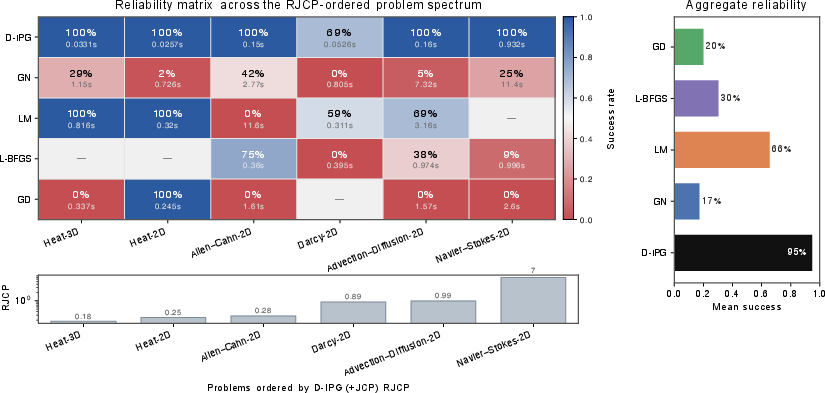
Abstract: Nonlinear inverse problems often trade inexpensive but fragile first-order updates against curvature-aware methods such as Gauss-Newton and Levenberg-Marquardt, which obtain stronger directions by repeatedly solving Jacobian-based linearized systems. We propose a learned alternative: amortize local inverse geometry into a reusable reverse operator. Our framework learns a bidirectional surrogate, Deceptron, and deploys it through D-IPG (Deceptron Inverse-Preconditioned Gradient), an iterative solver that pulls residual-corrected measurement-space proposals back to latent space. The key mechanism is a Jacobian Composition Penalty (JCP), which trains the reverse Jacobian to act as a local left inverse of the forward Jacobian; its runtime counterpart, RJCP, measures the same inverse-consistency error along optimization trajectories. We prove that D-IPG is first-order equivalent to damped Gauss-Newton under local pseudoinverse consistency, with deviation controlled by composition error and conditioning. Across seven PDE inverse-problem benchmarks, D-IPG outperforms standard baselines, achieves 94.8% mean success across the six-problem reliability suite, and reaches comparable or better recovery quality at up to 77x lower inference-time solve cost on the main benchmarks.
Paper Prompts
Sign up for free to create and run prompts on this paper using GPT-5.
Top Community Prompts
Explain it Like I'm 14
What is this paper about?
This paper is about solving “inverse problems” faster and more reliably by learning how to quickly “undo” a complicated process. Instead of repeatedly doing heavy math at every step (like classic methods do), the authors train a small helper model that learns the local rules for reversing the process. Then they plug this helper into a safe, step-by-step solver to find the hidden cause behind observed data.
They call the learned helper Deceptron and the overall solver D-IPG (Deceptron Inverse-Preconditioned Gradient).
What questions are the authors asking?
- Can we “learn once, use many times” the local geometry needed to undo a complex forward process, so that future inverse problems solve much faster?
- Can a learned reverse operator provide update directions that are as good as strong classical methods (like Gauss–Newton or Levenberg–Marquardt) but at a much lower cost?
- How do we train and check that this learned reverse operator really acts like a good local inverse?
How did they do it? (Methods explained simply)
First, a quick picture of inverse problems:
- Forward problem: You start with a hidden cause x (like the initial temperature of a metal bar) and a known simulator f that predicts what you can measure y (like temperatures you see later). This is “x → y.”
- Inverse problem: You observe y and want to find x. That’s harder: “y → x.”
What they build:
- A forward surrogate f_W: a neural network that mimics the real simulator but runs fast.
- A reverse map g_V: another neural network that tries to map measurements back to the hidden cause.
Key idea:
- Don’t try to perfectly invert the whole process everywhere. Instead, learn how to locally “undo” small changes: if you nudge the input x a bit, how does the output y change? And can the reverse map undo that small change? This “how things change” information is called the Jacobian. Think of it as a table of sensitivities: how much each output moves when each input wiggles.
Jacobian Composition Penalty (JCP):
- To teach g_V to be a good local undoer, they use a training penalty that encourages “do then undo ≈ do nothing” for small changes.
- In symbols: J_g(f(x)) * J_f(x) ≈ I (I = identity, meaning perfect canceling).
- You can think of it as pressing “do” followed by “undo,” and training so that the result is “back where you started.”
- There’s also a runtime version called RJCP that measures how well this property holds during solving.
The D-IPG solver (how a single step works):
- Start with a current guess x_t.
- Predict the measurement y_t = f_W(x_t).
- Compute the error r_t = y_t − y* (difference between prediction and the real observation).
- Move the measurement toward the target: y_prop = y_t − α r_t (α is a step size).
- Map back to the hidden space: x_prop = g_V(y_prop).
- Only accept the step if it actually reduces the objective (a “safety check” called Armijo backtracking). If not, try a smaller step.
Why this helps:
- Step 4 makes a sensible change in measurement space (push predictions toward what we saw).
- Step 5 uses the learned reverse operator to “pull” that change back into the hidden space.
- If g_V has learned good local inverse behavior, this produces smart, stable steps—similar to what strong classical methods compute by solving expensive linear systems.
Relation to Gauss–Newton (classic method):
- Gauss–Newton uses the Jacobian to find strong update directions but must solve a new linear system at every step (costly).
- The authors prove that if g_V’s Jacobian is a good local left-inverse of the forward Jacobian, then D-IPG’s update is, to first order, the same as a damped Gauss–Newton step—without solving that expensive system each time.
- How close D-IPG is to Gauss–Newton depends on:
- Composition error: how close J_g(f(x)) * J_f(x) is to identity.
- Conditioning: how stable the forward Jacobian is (ill-conditioned = tricky/problematic).
What did they find?
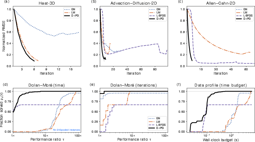
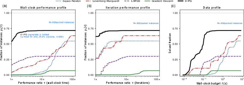
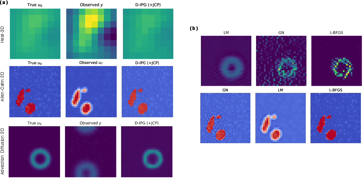
Across seven inverse problems based on physical systems (PDEs like heat flow, fluid dynamics, and more):
- D-IPG often reaches similar or better solution quality than strong classical methods but much faster—up to 77× less compute at inference time on the main benchmarks.
- It beats common first-order baselines and is competitive with second-order methods while being cheaper per iteration.
- On a six-problem “reliability suite,” it succeeds on average 94.8% of the time, more uniformly than the baselines.
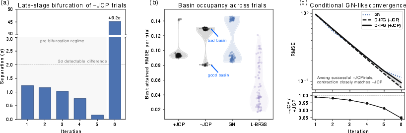
Why JCP matters:
- With JCP, many more runs enter the “good basin” (the region where the solver can rapidly refine the correct solution). Once in that basin, even the version without JCP contracts similarly—but JCP gets you there much more often. In short, JCP boosts reliability and basin access.
Where it struggled:
- One problem (Darcy-2D) is very ill-conditioned. The theory predicts that when conditioning is bad and composition error isn’t tiny, the learned direction can deviate more from Gauss–Newton, reducing reliability. That’s exactly what they observe.
Why is this important?
- Inverse problems show up everywhere: medical imaging, climate and weather, engineering design, and geophysics. These are often repeated many times with similar physics.
- This paper shows you can “amortize” (learn once, reuse many times) the expensive local inverse geometry so that future solves are much faster.
- You keep the safety of a proper optimizer (accept only steps that help), but you get the speed of a learned helper.
What are the implications and limitations?
Implications:
- Faster, more reliable inverse solves for families of related problems.
- A practical bridge between traditional math-heavy optimization and modern learned components.
- A clear training target (JCP) and a runtime diagnostic (RJCP) so you can tell when to trust the learned reverse geometry.
Limitations:
- If the learned forward surrogate is poor, the reverse won’t fix it.
- The “Gauss–Newton-like” guarantee is local; it doesn’t ensure global convergence.
- Best payoff comes when you solve many similar problems (amortization). For one-off problems, the training cost may not be worth it.
Overall, the paper’s main message is simple but powerful: the tricky “local rules for undoing” a process don’t have to be rebuilt from scratch each time—you can learn them once and apply them quickly and safely inside a standard solver.
Knowledge Gaps
Knowledge gaps, limitations, and open questions
Below is a single, concise list of concrete gaps and unresolved questions that future work could address:
- Global guarantees: Only local, first-order equivalence to (damped) Gauss–Newton is shown. What verifiable conditions on JCP/RJCP, step-size/backtracking, relaxation, and projection ensure global convergence and convergence rates?
- Armijo acceptance under amortization: When and why does Armijo backtracking reliably accept D-IPG steps generated by a learned reverse map? Can one prove eventual acceptance and sufficient decrease under bounded RJCP and Lipschitz assumptions, including the effects of projection and relaxation?
- Handling rank deficiency and underdetermined regimes: Theory assumes full column rank of the forward Jacobian. How should JCP and D-IPG be modified for rank-deficient or severely under/overdetermined problems, e.g., by training a damped pseudoinverse, projecting JCP onto the Jacobian range, or explicitly regularizing null-space components?
- Ill-conditioning robustness: In highly ill-conditioned settings (e.g., Darcy-2D), composition error is amplified. Can JCP be reformulated to target a damped pseudoinverse (LM-like) family, e.g., training G ≈ (JT J + λI){-1} JT with adaptive λ, and can RJCP be extended to diagnose and control such damping online?
- Surrogate-to-physics gap: Inference and acceptance are performed against the learned surrogate f_W. How does mismatch between f_W and the true forward model bias recovery, and can a hybrid loop (e.g., surrogate-driven steps with periodic checks or corrections using the true solver) mitigate this?
- RJCP as an adaptive controller: RJCP is used diagnostically, not algorithmically. What thresholds reliably predict failure, and how can RJCP trigger safeguards (e.g., fallback to GN/LM, reduced step sizes, increased relaxation, or on-the-fly reweighting of residual corrections)?
- Data efficiency and sample complexity: How many (x, y) pairs and what coverage of the Jacobian spectrum are required for g_V to generalize its local inverse action? Can one derive sample-complexity bounds or curricula for Jacobian coverage?
- Probe design for JCP: JCP uses Hutchinson probes to control a Frobenius-norm composition defect. How many probes are needed to bound spectral error with high probability, and can probe directions be adaptively chosen (e.g., aligned with dominant residual/Jacobian subspaces) to improve training efficiency?
- Noise models and robustness: The method optimizes unweighted least squares. How does performance change under heteroscedastic or correlated measurement noise, and can JCP/RJCP and the D-IPG proposal be extended to weighted/robust losses (e.g., Huber, Cauchy) and known noise covariances?
- Constraints and projection: The projection set C and operator Π_C are assumed but not characterized. How does D-IPG behave with nonconvex or expensive-to-project constraints, and can feasibility be maintained with alternative safegaurds (e.g., barrier/penalty methods) while preserving the learned inverse geometry?
- Architecture choices and stability: What network classes (e.g., invertible/bi-Lipschitz architectures, spectral normalization, monotone networks) best preserve stable local inverse geometry and small RJCP, especially in high-dimensional PDE settings?
- Scaling and memory: What are the practical limits of D-IPG when d_in and d_out are very large (e.g., 3D high-resolution fields)? How do JVP/VJP costs, RJCP evaluation, and training-time JCP scale, and what batching or low-rank approximations mitigate memory/runtime growth?
- Beyond PDEs and domain shift: Generalization is shown across PDE inverse problems from a shared family. How well do learned reverse maps transfer across different PDEs, boundary conditions, mesh resolutions, or sensor layouts, and what adaptation is required under domain shift?
- Real-data validation: Experiments are on synthetic PDE benchmarks. How does the approach perform with real measurements (noise, model error, discretization mismatch), and can physics-consistent acceptance tests or mixed-fidelity training mitigate real-world discrepancies?
- Amortization economics: Reported speedups exclude training cost. What is the break-even analysis (instances needed to amortize training) as a function of problem size, conditioning, and target accuracy, and how do these trade-offs compare against classical solvers with warm starts?
- Hybridization with classical solvers: Can one design principled hybrids that interleave D-IPG steps with occasional GN/LM solves to recalibrate g_V (online or episodically), especially when RJCP spikes or basin-entry fails?
- Multi-step or trust-region variants: Residual correction uses y_prop = y − α r. Would anisotropic or learned measurement-space corrections (e.g., learned metric or trust region in y-space) improve stability and basin entry; how should these be trained and safeguarded?
- Iteration-wise error propagation: Theorems bound single-step deviations. Can one bound cumulative deviation and establish iteration-level convergence guarantees that relate RJCP trajectories to final reconstruction error?
- Adaptivity and online fine-tuning: Can g_V be updated online per instance (e.g., via low-rank Jacobian corrections) without destroying acceptance safeguards, and does such adaptation improve reliability on hard instances like Darcy-2D?
- Coverage diagnostics for training: Beyond RJCP, can we devise training-time diagnostics that ensure adequate coverage of the local Jacobian manifold that will be encountered at inference (e.g., curriculum sampling of x, adversarial residual directions)?
- Handling non-injective forwards: When the forward map is non-injective, multiple x map to similar y. How should JCP and D-IPG incorporate priors, regularization, or Bayesian uncertainty to disambiguate solutions while maintaining stable inverse geometry?
- Weighted objectives and priors: Can D-IPG be extended to regularized or MAP formulations (e.g., Φ(x) + λΨ(x)) with priors Ψ, and can JCP be adapted to respect the induced metric (e.g., Gauss–Newton in the prior-preconditioned geometry)?
- Comparative baselines: The study does not compare against modern learned/unrolled inverse methods or operator-learning baselines used as iterative preconditioners. How does D-IPG fare against these alternatives under matched training budgets and solve-time constraints?
- Failure-mode analysis: Heat-1D failure mode is noted but not dissected. What specific properties (architecture, data coverage, conditioning, discretization) caused f_W to “fail to expose reliable local inverse structure,” and which interventions fix it (e.g., data augmentation, architectural constraints, modified JCP)?
- Hyperparameter guidelines: Practical guidance is limited for α, ρ, JCP weights, and probe counts. Can we provide principled selection rules tied to conditioning estimates, RJCP levels, or problem scales to reduce tuning effort?
Practical Applications
Immediate Applications
Below are concrete ways the paper’s ideas can be deployed now, given the released codebase, the method’s reliance on standard autodiff tooling, and the empirical evidence of speedups and reliability.
- Healthcare — Imaging reconstruction and parameter estimation
- Use case: Faster iterative MRI/CT/PET reconstruction pipelines in research hospitals and imaging labs, replacing repeated Gauss–Newton/LM solves with D-IPG to cut wall-clock per reconstruction while preserving safeguards (Armijo backtracking).
- Product/workflow: A “D-IPG recon” plugin for open-source frameworks (e.g., Gadgetron, BART, SigPy), with an RJCP dashboard to monitor learned inverse quality during deployment.
- Assumptions/dependencies: Availability of a differentiable forward surrogate for the scanner’s physics; sufficiently many historical instances to amortize training; stable operating regime (limited distribution shift); compliance pipeline for clinical research use only (not clinical diagnosis without further validation).
- Energy and subsurface — PDE-constrained inversion (Darcy flow, geothermal, seismic pre-stack)
- Use case: Accelerate ensemble-based reservoir characterization and pre-production screening by amortizing local inverse geometry; use RJCP to decide when to fall back to LM on ill-conditioned cases.
- Product/workflow: A preconditioned solver module that wraps existing inversion suites (e.g., PETSc/TAO, FEniCS/Firedrake workflows) and selects D-IPG when RJCP is below a threshold, else defers to classical solvers.
- Assumptions/dependencies: Good surrogate fidelity to the simulator; problem families recur (amortization benefit); ill-conditioning can be high (as observed on Darcy-2D), so a hybrid “RJCP-triggered fallback” is needed.
- Advanced manufacturing and non-destructive testing
- Use case: Speed up iterative CT-based quality assurance, ultrasonic/eddy-current inversion for defect detection, and process-parameter recovery in additive manufacturing.
- Product/workflow: A “learned inverse geometry” service that trains JCP-enabled Deceptrons on past parts and deploys D-IPG at the edge on production lines; Armijo safeguards ensure descent on the explicit defect objective.
- Assumptions/dependencies: Access to synthetic or measured paired data; stable acquisition settings; retraining when sensors or materials change significantly.
- Robotics and automation — Calibration and system identification
- Use case: Faster calibration of camera–lidar rigs, manipulator dynamics parameter fitting, and soft-robot model identification where the forward map is differentiable or surrogated.
- Product/workflow: A D-IPG “calibration accelerator” that plugs into existing toolchains (Kalibr/ceres-solver-based stacks) and reduces solve time for repeated, factory-scale calibration tasks.
- Assumptions/dependencies: Differentiable surrogate of the sensor/actuator stack; many similar calibration instances (amortization); guardrails for out-of-distribution motions.
- Scientific computing and academia — PDE inverse problems and teaching
- Use case: Replace repeated linear solves in Gauss–Newton with amortized reverse operators for heat, advection–diffusion, Allen–Cahn, Navier–Stokes parameter recovery (as in the paper’s benchmarks).
- Product/workflow: Integrate the provided PyTorch implementation into research codes; use RJCP to track local inverse consistency across optimization trajectories and log solver diagnostics for papers.
- Assumptions/dependencies: Autodiff access (JVPs/VJPs) to compute JCP cheaply; training time is amortized across many problem instances.
- Software engineering — Solver acceleration libraries
- Use case: Ship a reusable “inverse-preconditioned gradient” layer in ML frameworks that can wrap arbitrary differentiable forward models to provide D-IPG steps with Armijo line search.
- Product/workflow: A pip-installable package exposing Deceptron modules, D-IPG optimizer, and RJCP metrics; CI tests verifying JCP reductions and GN-direction equivalence on toy problems.
- Assumptions/dependencies: Consistent API for forward models and feasibility projections; users provide task/data and choose acceptance constants (Armijo c, backtracking β).
- Remote sensing and computational photography
- Use case: Faster iterative deblurring, super-resolution, and hyperspectral unmixing where classic solvers are robust but slow; D-IPG amortizes per-instance geometry across a device class.
- Product/workflow: A camera/processing pipeline module that runs a few D-IPG iterations with α≈1, optionally switching to TV-regularized LM when RJCP rises or residual reduction stalls.
- Assumptions/dependencies: Stable optics and noise statistics (per device class); forward model differentiability; privacy-safe training data or high-fidelity simulators.
- Operations and monitoring — On-line inverse updates for digital twins
- Use case: Near-real-time parameter tracking in thermal, fluid, or structural digital twins by pulling measurement residuals back to latent states without solving new linear systems each cycle.
- Product/workflow: Embed D-IPG as a loop in the twin’s update step; log RJCP and residual ratios to trigger recalibration when learned geometry drifts.
- Assumptions/dependencies: Twin fidelity and differentiability; sufficient stationarity to justify amortization; watchdog to handle drift.
Long-Term Applications
These applications require further research, scaling, validation, or tooling to meet robustness, regulatory, or system-integration needs.
- Healthcare (regulated) — Certified, real-time clinical reconstruction
- Use case: FDA/CE-cleared D-IPG-powered recon for MRI/CT/PET and interventional imaging with strict safety/quality guarantees.
- Product/workflow: A certifiable reconstruction stack with formal RJCP thresholds, automated fallbacks to LM, uncertainty estimation, and prospective clinical trials.
- Assumptions/dependencies: Regulatory evidence; robust distribution-shift handling; standardized RJCP-based acceptance criteria; dataset shift monitoring and periodic revalidation.
- Weather, ocean, and climate — Data assimilation preconditioning (4D-Var/EnKF)
- Use case: Use learned reverse geometry to precondition incremental 4D-Var updates, reducing wall-clock in operational NWP and ocean reanalyses.
- Product/workflow: A hybrid assimilation engine that queries g_V for observation-space residual pullbacks and switches to classical linear solvers when RJCP flags instability.
- Assumptions/dependencies: Differentiable surrogates of observation operators and models (or operator-learning proxies like FNO/DeepONet); massive-scale training; rigorous stability margins.
- Seismic full-waveform inversion at basin scale
- Use case: Amortize local inverse geometry across survey patches to reduce per-iteration PDE solves, improving turnaround time for exploration campaigns.
- Product/workflow: Multi-resolution Deceptrons co-trained with operator-learning surrogates; adaptive RJCP gating across depth/frequency bands.
- Assumptions/dependencies: High-fidelity surrogates for complex geology; multi-fidelity training; integration with HPC workflows and checkpointing.
- Real-time control with differentiable digital twins
- Use case: Closed-loop control where D-IPG provides fast latent-state corrections enabling MPC at higher rates for thermal/HVAC, microgrids, and process plants.
- Product/workflow: A controller that alternates D-IPG state correction with control optimization; safety envelope enforced by projection Π_C and fallback controllers when RJCP degrades.
- Assumptions/dependencies: Robustness to disturbances; verifiable safety under model mismatch; embedded acceleration (GPU/TPU/ASIC).
- Robotics — Embedded, certifiable calibration and system ID
- Use case: On-robot, on-boot calibration for fleets, with learned inverse geometry shared across robots and RJCP-based self-diagnosis for maintenance.
- Product/workflow: Fleet-wide “inverse geometry models” over-the-air updated; devices self-check RJCP and flag recalibration or service.
- Assumptions/dependencies: Hardware acceleration for autodiff; secure update channels; formal bounds on deviation and safe fallbacks.
- Foundation models for inverse problems
- Use case: Pretrain a general-purpose Deceptron over families of PDEs/forward operators to deliver broadly transferable local inverse geometry.
- Product/workflow: A model zoo with task adapters; meta-learning to specialize g_V quickly; standardized RJCP tests across domains.
- Assumptions/dependencies: Large, diverse synthetic corpora; scalable JCP training with efficient JVPs/VJPs; benchmarks and community standards.
- Policy and standards — Trust metrics for learned solvers
- Use case: Establish RJCP-like diagnostics as reportable metrics in industry/medical/energy standards to certify the reliability of learned components inside optimization pipelines.
- Product/workflow: Reference implementations, test suites, and conformance criteria that tie acceptable RJCP ranges to convergence guarantees and fallback policies.
- Assumptions/dependencies: Multi-stakeholder consensus; reproducible benchmarks; mapping from RJCP thresholds to risk categories.
- Privacy-preserving, on-device inverse inference
- Use case: Perform imaging and sensing inversions on-device (phones, wearables, drones) with D-IPG’s low iteration count and no cloud dependency.
- Product/workflow: Quantized/compiled Deceptron models (e.g., via TensorRT/TVM) and low-rank JCP training to fit memory/power constraints.
- Assumptions/dependencies: Efficient JVP/VJP kernels on edge hardware; domain-specific surrogates; careful thermal/power budgeting.
- Automated solver orchestration
- Use case: Systems that learn when to use D-IPG vs. LM/GN/L-BFGS per-instance based on RJCP, residual structure, and estimated conditioning.
- Product/workflow: A scheduler that estimates σ_min(J) proxies and uses RJCP to route instances; logs outcomes to continually refine routing policies.
- Assumptions/dependencies: Reliable conditioning estimators; guardrails to avoid oscillation; audit trails for high-stakes applications.
- Data-efficient and active learning for JCP
- Use case: Reduce training cost by selecting probes and instances that most reduce composition error where solvers operate.
- Product/workflow: An active JCP trainer that samples along solver trajectories, prioritizing high-RJCP regions to tighten the Gauss–Newton deviation bound.
- Assumptions/dependencies: Online data collection; safe exploration; curriculum over operating regimes.
Cross-cutting dependencies and assumptions
- Amortization regime: Benefits are largest when many inverse instances share the same forward family; one-off problems may not justify training cost.
- Differentiable surrogate fidelity: f_W must expose the relevant local geometry; poor surrogates limit D-IPG reliably (observed in Heat-1D).
- Conditioning: Ill-conditioned problems can amplify deviations; RJCP and fallback strategies are important (theory and Darcy-2D results).
- Safeguards: Armijo backtracking, projection Π_C, and relaxation ρ are integral to stability; α=1 is natural but must be guarded.
- Distribution shift: g_V is local; monitor RJCP to detect drift and trigger retraining or solver fallback.
- Compute and tooling: Access to autodiff (JVPs/VJPs), GPU acceleration for training, and integration with existing solver stacks.
These applications leverage the paper’s core innovations—amortized reverse operators (Deceptron), the D-IPG solver, and JCP/RJCP as training-time and runtime mechanisms—to move trusted second-order geometry into a reusable, monitored component, yielding strong speedups and reliability in recurring inverse problems.
Glossary
- Advection–diffusion: A partial differential equation modeling transport combining directed flow (advection) and spreading (diffusion). Example: "advection--diffusion, Allen--Cahn, and Navier--Stokes inversion."
- Allen–Cahn: A reaction–diffusion PDE modeling phase separation and interface motion. Example: "Allen--Cahn"
- Amortized: Learned once and reused across instances or iterations rather than recomputed each time. Example: "amortize local inverse geometry into a reusable reverse operator."
- Armijo backtracking: A line-search method that ensures sufficient decrease of the objective by shrinking the step size until a condition is met. Example: "Armijo backtracking is used as an acceptance safeguard"
- Basin occupancy: The fraction of runs that enter a particular basin of attraction (e.g., low-error region). Example: "studies basin occupancy on Allen--Cahn-2D"
- Cohen's d: A standardized effect-size measure quantifying separation between groups. Example: "using Cohen's "
- Cycle consistency: A training constraint encouraging that mapping forward then backward (or vice versa) approximately recovers the original input. Example: "cycle-consistency terms anchor the reverse map"
- D-IPG (Deceptron Inverse-Preconditioned Gradient): The proposed iterative solver that pulls residual-corrected measurement proposals back to latent space using a learned reverse map. Example: "D-IPG (Deceptron Inverse-Preconditioned Gradient)"
- Damped Gauss–Newton: A Gauss–Newton variant with damping to improve robustness, akin to Levenberg–Marquardt. Example: "first-order equivalent to damped Gauss--Newton"
- Darcy flow: An elliptic PDE governing flow through porous media. Example: "including Darcy flow"
- DeepONets: Neural architectures for learning operators mapping between function spaces. Example: "DeepONets and Fourier neural operators"
- Fourier neural operators: Operator-learning architectures using Fourier transforms to learn mappings between function spaces. Example: "Fourier neural operators"
- Frobenius norm: The square root of the sum of the squares of all matrix entries; equivalent to the Euclidean norm of the matrix viewed as a vector. Example: "exactly in Frobenius norm."
- Gauss–Newton: A second-order method for nonlinear least squares that solves linearized systems using the Jacobian. Example: "Gauss--Newton"
- Hutchinson's estimator: A stochastic method to estimate matrix traces (and related quantities) using random probe vectors. Example: "By Hutchinson's estimator"
- Ill-conditioned: Having poor numerical conditioning (e.g., large condition number), leading to instability or slow convergence. Example: "when the forward Jacobian is ill-conditioned"
- Jacobian: The matrix of first derivatives of a vector-valued function with respect to its inputs. Example: "forward Jacobian"
- Jacobian Composition Penalty (JCP): A training objective that penalizes deviation of the reverse–forward Jacobian composition from the identity to enforce local inverse consistency. Example: "Jacobian Composition Penalty (JCP)"
- Jacobian-vector product (JVP): The product of a Jacobian with a vector, efficiently computed via automatic differentiation. Example: "JVPs compute "
- Levenberg–Marquardt: A damped Gauss–Newton algorithm blending gradient descent and Gauss–Newton for robust nonlinear least squares. Example: "Levenberg--Marquardt"
- Moore–Penrose pseudoinverse: A generalized matrix inverse providing least-squares solutions, especially for non-square or rank-deficient matrices. Example: "the Moore--Penrose pseudoinverse"
- Navier–Stokes: The PDEs governing fluid dynamics. Example: "Navier--Stokes inversion"
- Operator learning: Learning mappings between function spaces (operators), rather than finite-dimensional vectors. Example: "operator-learning approaches"
- Preconditioners: Transformations applied to linear or nonlinear systems to improve conditioning and accelerate iterative solvers. Example: "learned preconditioners aim to accelerate iterative linear solves."
- Projection onto a feasible set: Mapping a point to the closest point within a constrained set. Example: "projection onto a feasible set "
- Quasi-Newton: Optimization methods that approximate second-order information (Hessian) to achieve faster convergence than first-order methods. Example: "quasi-Newton procedures"
- Range (of a matrix): The subspace spanned by a matrix’s columns (its image). Example: ""
- Relaxation parameter: A scalar blending current and proposed iterates to stabilize updates. Example: " is a relaxation parameter."
- Reverse-mode differentiation: An automatic differentiation technique (backpropagation) efficient for functions with many inputs and few outputs. Example: "reverse-mode differentiation backpropagates the resulting probe-based losses."
- RJCP (runtime Jacobian Composition Penalty): A diagnostic measuring the same inverse-consistency error as JCP along optimization trajectories. Example: "RJCP, measures the same inverse-consistency error"
- Smallest singular value: The minimum singular value of a matrix, governing local conditioning and stability. Example: "the smallest singular value of "
- Spectral norm: The largest singular value of a matrix; the operator 2-norm. Example: "induced spectral norms"
- Surrogate (forward surrogate): A learned differentiable approximation of the forward model used during training and inference. Example: "forward surrogate"
- Taylor's theorem: A result that approximates a function near a point using derivatives, providing error terms. Example: "Taylor's theorem gives"
- Unrolled optimization: Learned architectures that mimic a fixed number of iterations of an optimization algorithm. Example: "unrolled optimization methods"
Collections
Sign up for free to add this paper to one or more collections.