Budget Constraints as Riemannian Manifolds
Abstract: Assigning one of K options to each of N groups under a total cost budget is a recurring problem in machine learning, appearing in mixed-precision quantization, non-uniform pruning, and expert selection. The objective (model loss) depends jointly on all assignments and does not decompose across groups, which prevents combinatorial solvers from optimizing the true objective directly and limits them to proxy objectives. Evolutionary search evaluates the actual loss but lacks gradient information, while penalty-based methods provide gradients but enforce the budget only approximately and require sensitive hyperparameter tuning. We observe that under softmax relaxation, the budget constraint defines a smooth Riemannian manifold in logit space with particularly simple geometry: the normal vector is available in closed form, shifting logits along the cost vector changes expected cost monotonically, allowing binary-search retraction, and vector transport reduces to a single inner product. Building on this structure, we propose Riemannian Constrained Optimization (RCO), which augments a standard Adam update with tangent projection, binary-search retraction, and momentum transport. Combined with Gumbel straight-through estimation and budget-constrained dynamic programming for discrete feasibility, RCO enables first-order optimization of the true objective under exact budget enforcement, without introducing constraint hyperparameters. On synthetic knapsack problems with known optima, the manifold-based constraint handling recovers optimal solutions, whereas penalty methods plateau at 83% of optimal. On LLM compression tasks, including mixed-precision quantization and MoE expert pruning, RCO matches or exceeds evolutionary search methods while requiring 3x to 16x lower wall-clock cost on the evaluated configurations.
Paper Prompts
Sign up for free to create and run prompts on this paper using GPT-5.
Top Community Prompts
Explain it Like I'm 14
What this paper is about (big picture)
Imagine you’re packing a backpack with a strict weight limit. You have lots of items (like snacks, clothes, tools), and for each item you must choose one version (light, medium, or heavy). You want the best overall trip experience, but you cannot go over the weight limit.
This paper tackles the same kind of problem in machine learning: choosing, for each part of a big model, one option (like how many bits to use or whether to keep/prune a component) so that:
- the model stays within a total “budget” (like size, speed, or memory), and
- the model’s performance stays as good as possible.
Their core idea is to treat the exact budget limit as a smooth surface you can “walk on” while optimizing, so the budget is always exactly respected—no guessing or penalty tuning needed.
What questions the authors ask
- Can we pick options for many parts of a model so we hit an exact total budget (not just approximately) while still using fast, gradient-based training?
- Can we avoid slow, guess-and-check methods (like evolutionary search) and also avoid penalty tricks that often overshoot or undershoot the budget?
- Can we make this work on real tasks like compressing LLMs without losing too much quality?
How their method works (in everyday terms)
Think of all possible option choices as a big control panel with many sliders. Each slider controls how likely you are to pick a certain option for a given part (e.g., a layer’s bitwidth). These sliders produce:
- probabilities for each option (using a standard tool called “softmax”), and
- an expected total “cost” (like total model size).
Now, picture all slider settings that exactly meet the budget as forming a smooth “surface” in space. The authors:
- Move along this surface in directions that improve the model without changing the total cost (this is like sliding sideways along a hill at the same height—staying on the same “budget level”).
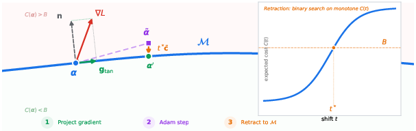
- If a move drifts slightly off the surface (because optimizers like Adam rescale steps), they nudge back to the surface by turning one special knob that raises or lowers the overall cost in a predictable way. They use binary search—like moving left or right until the cost matches the budget exactly.
- They also adjust the optimizer’s “momentum” so it keeps pointing along the surface after each nudge.
To actually test the model with real, discrete choices (not just probabilities), they do two complementary things:
- Forward pass (testing): Use a clever randomizer (Gumbel) and a fast “smart packing” algorithm (dynamic programming for knapsack) to pick a concrete set of options that fits the budget exactly.
- Backward pass (learning): Use a “straight-through estimator” to send gradient information back through those discrete choices, then project that gradient so it never pushes away from the budget.
Why this is neat:
- The “budget surface” has a very clean geometry. The direction that changes total cost (the “normal”) is simple to compute, and the “retraction” (nudging back onto the surface) is just a quick binary search along a single direction.
- No extra penalty knobs to tune. The budget is satisfied exactly at every step.
What they found and why it matters
On toy problems where the best answer is known (multiple-choice knapsack):
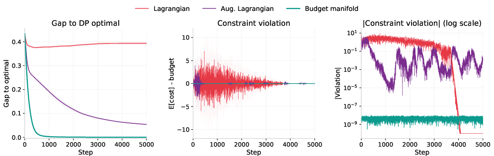
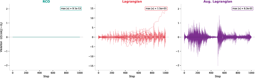
- Their method hits the exact budget (down to tiny numerical error) and finds optimal or near-optimal solutions.
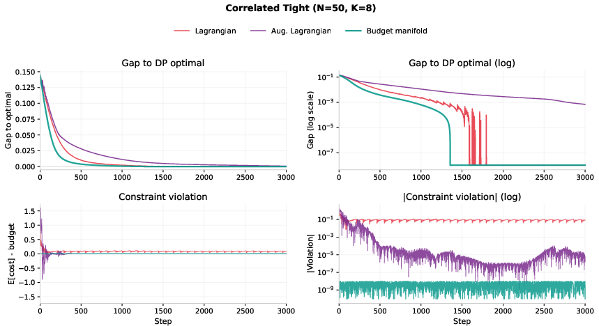
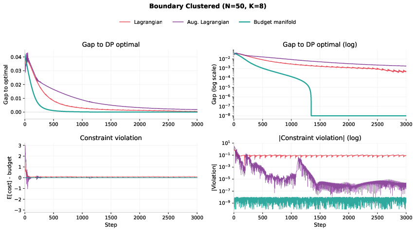
- Standard penalty or Lagrangian methods often keep violating the budget and get stuck at only about 83% of the best possible score on tough cases.
On real model compression tasks:
- Mixed-precision quantization (choosing bits per layer) and MoE expert pruning (choosing which experts to keep/drop):
- Their method matches or beats evolutionary search methods while being 3–16× faster in the tests they ran.
- At very high compression (very tight budgets), it outperforms methods that rely on simple per-layer scores or surrogates, which can break down.
Why it’s important:
- Exact budget control is valuable for deploying AI on devices with strict limits (phones, edge devices, specific servers).
- Saving time (fewer model evaluations) means cheaper, faster iteration and tuning.
- Avoiding fragile penalty settings makes the process more reliable.
What this could change (impact and limitations)
- Impact:
- Provides a practical way to make large models smaller or faster without guessing penalty strengths or running slow search for hours.
- Offers precise control: you decide the budget, and the optimizer respects it at every step.
- Can be combined with different optimizers and tasks since it’s a “wrapper” around standard gradient methods.
- Limitations to keep in mind:
- The forward “smart packing” step (dynamic programming) depends on budget discretization and the number of options; with huge option sets, it could become a bottleneck.
- The technique relies on costs being a simple linear combination of choices. If the true cost is nonlinear (like complicated latency), the “simple nudge back” trick may need adjustments.
- The gradient through discrete choices (straight-through estimator) is an approximation; while the method works well in practice, full theoretical guarantees for the whole system are limited.
In one sentence
The paper shows how to turn the “stay under budget” rule into a smooth surface you can safely walk along while training, letting you choose the best options across a model exactly within budget—fast, reliable, and often better than common alternatives.
Knowledge Gaps
Knowledge gaps, limitations, and open questions
The paper proposes a Riemannian treatment of budget constraints and demonstrates promising empirical results. The following concrete gaps and open problems remain for future work:
- Convergence with biased gradients: Provide theoretical guarantees (or counterexamples) for RCO when gradients come from Gumbel-STE and Adam with temperature annealing on the budget manifold; current convergence claims apply only to exact gradients.
- Bias after projection: Quantify how much STE bias remains after tangent projection (beyond the normal component) and how this residual bias affects convergence rate and solution quality.
- Retraction near saturation: Analyze numerical stability and bracketing strategies for binary-search retraction when concentrate (variance ), which makes arbitrarily small and can slow root finding.
- Beyond linear expected-cost constraints: Extend the geometric framework to nonlinear or non-additive costs (e.g., latency, energy, or bandwidth models) where shifting logits by no longer yields monotonic ; develop valid retraction schemes for such constraints.
- Per-group costs and heterogeneous option sets: Generalize the manifold and retraction to costs (option costs varying by group), or to group-specific option sets , and characterize when the monotonic retraction still holds.
- Multiple constraints in practice: The multi-constraint projection is outlined, but there is no empirical evaluation; study numerical conditioning when normals are nearly colinear, retraction strategies for , and effects on optimizer stability.
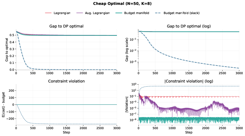
- Inequality constraints via slack: The slack-variable construction is introduced but not validated on LLM tasks; evaluate how often optimal solutions leave slack , how to schedule/regularize , and whether slack induces undesirable degeneracies.
- DP scalability and discretization: Assess forward-pass DP cost for large or fine budget discretization ; evaluate approximation-quality vs. speed trade-offs for coarser discretization or alternative solvers (e.g., FPTAS, Lagrangian DP, or learned surrogates).
- Discretization error and manifold mismatch: Study the impact of discretizing the budget in DP while enforcing exact expected cost in the backward pass, including conditions under which expected-cost feasibility misaligns with discrete feasibility and how to mitigate.
- Alternative differentiable combinatorial solvers: Compare STE to differentiable optimization approaches (e.g., perturbation-based, KKT-based, or implicit differentiation through knapsack/MCKP) for bias–variance trade-offs and sample efficiency.
- Sample efficiency and variance reduction: Systematically analyze and design variance-reduction methods (e.g., control variates, antithetic Gumbels, Rao–Blackwellization) that reduce the need for large Gumbel sample counts per step without degrading convergence.
- Temperature schedules: Provide principled guidelines (or adaptive schemes) for temperature annealing to balance exploration and stability, and study failure modes from overly aggressive or conservative schedules.
- Initialization sensitivity: Evaluate how initialization of logits (e.g., from REAP or uniform) affects convergence and local minima, and whether warm starts or meta-initialization improve outcomes across budgets.
- Equal or nearly equal costs: Investigate behavior and regularization strategies when many options share identical or nearly identical , which can lead to small or ill-conditioned normals and slow manifold updates.
- Cost scaling and conditioning: Examine sensitivity to the scale of and (e.g., whether normalization improves conditioning of projection and retraction, or interacts adversely with Adam’s adaptive scaling).
- Retraction step improvements: Explore Newton or safeguarded Newton methods for scalar retraction with analytic derivatives (and possibly second derivatives), characterize basin sizes, and compare to binary search in speed and robustness.
- Momentum transport choices: Compare projection-based vector transport to alternative transports (e.g., pole ladder) and assess impacts on optimizer momentum and convergence, especially under curvature.
- Second-order methods on the manifold: Investigate Riemannian quasi-Newton or natural-gradient methods tailored to the budget manifold and compare their convergence speed and stability to Adam-based RCO.
- Interaction with adaptive optimizers: Characterize how per-coordinate scaling (Adam, Adagrad) interacts with projection/retraction and whether manifold-aware preconditioning yields consistent improvements.
- Memory overhead for quantization: For mixed-precision quantization, precomputing and storing per-layer weights/residuals for all bitwidths is memory-intensive; study incremental/on-the-fly quantization or low-rank residual parameterizations that reduce memory while preserving differentiability.
- Generalization to training-time constraints: Evaluate RCO during fine-tuning or training from scratch (not just post-training calibration) under dynamic budgets, and examine stability and generalization compared to post-training application.
- Multi-objective and compound constraints: Extend and empirically validate RCO with simultaneous constraints (e.g., model size, FLOPs, latency) and study trade-off surfaces and Pareto-front exploration on real hardware.
- Hardware-grounded costs: Replace proxy costs (bits/parameters) with measured latency/energy on specific devices and quantify how non-additivities (caches, operator fusion) affect feasibility and the viability of monotonic retraction.
- Broader domains: Test RCO beyond LLM compression (e.g., NAS, pipeline budgets, RL constraints) to validate generality and identify domain-specific adaptations required.
- Evaluation breadth and robustness: Expand empirical evaluation to more models, datasets, and higher compression regimes; report sensitivity analyses across seeds, calibration set sizes, and budget levels.
- Fair comparisons and compute accounting: Provide standardized budgets for wall-clock comparisons (same number of forward/backward passes, hardware) and ablate the DP/discretization overhead to isolate manifold vs. search contributions.
- Theoretical link between calibration KL and task metrics: Formalize when minimizing calibration KL (Eq. ) guarantees improvements in downstream metrics (accuracy, perplexity, coding pass@1), especially under significant compression.
- Guarantees for discrete final solutions: Establish conditions under which optimizing expected-cost-constrained logits via RCO yields discrete assignments close to the true constrained optimum, and bound the optimality gap induced by STE and DP discretization.
- Robustness to cost/model mismatch: Analyze sensitivity when the assumed cost model () is mis-specified relative to actual deployment costs, and develop robust or adaptive cost-estimation procedures within RCO.
Practical Applications
Overview
The paper introduces a geometric approach to budget-constrained discrete assignment problems—common in machine learning model compression—by treating the expected-cost level set under softmax as a smooth Riemannian manifold. The proposed Riemannian Constrained Optimization (RCO) algorithm integrates: (1) tangent projection to remove budget-violating gradient components, (2) a monotonic binary-search retraction that guarantees exact budget enforcement, and (3) momentum vector transport. In the forward pass, discrete feasibility is enforced via a budget-constrained multiple-choice knapsack dynamic program (DP) combined with Gumbel Straight-Through Estimation (STE) for differentiability; in the backward pass, the manifold ensures exact budget satisfaction with no constraint hyperparameters. Empirically, RCO reaches or exceeds the quality of evolutionary search with significantly lower wall-clock time on LLM compression and matches DP optima on synthetic knapsack benchmarks where penalty methods stall.
Below are practical, real-world applications derived from these findings, grouped by deployment horizon.
Immediate Applications
These applications can be deployed now with modest engineering effort, leveraging the paper’s assumptions (linear cost in selection probabilities, known discrete options and costs, feasible DP scale, availability of a calibration set).
- LLM post-training mixed-precision quantization under strict memory/size budgets (Software, Cloud/Edge)
- Use RCO to assign per-layer bitwidths (e.g., 2–8 bits) that minimize calibration loss while exactly meeting an average-bit or parameter-size budget; integrates with GPTQ/other PTQ backends.
- Tools/workflows: “RCO-Quantizer” module for PyTorch/Hugging Face Optimum; CI pipelines that auto-tune per-device budgets (A/B test across devices).
- Assumptions/Dependencies: Pre-quantized weight candidates per bitwidth; calibration dataset; linear cost proxy (bits/parameter) and known per-layer weights; DP discretization B′ manageable.
- MoE expert pruning with guaranteed global budgets (Software, Cloud Serving)
- Allocate prune/keep decisions across layers to hit global expert-count or memory/compute budgets, improving inference cost without violating constraints; RCO can deviate from per-layer heuristics (e.g., REAP) when the global loss favors it.
- Tools/workflows: “RCO-Pruner” for MoE; serving-time profiles to select budget-aware expert subsets for SKU tiers.
- Assumptions/Dependencies: Binary per-expert costs or known per-expert cost vector; calibration data; stable STE training; DP feasibility at expert counts.
- Non-uniform structured pruning under parameter or FLOPs budgets (Software, Mobile/Embedded)
- Select layer-wise sparsity levels from discrete menus while minimizing end-to-end loss; preserves budget exactly at every optimizer step.
- Tools/workflows: Integration with pruning frameworks (e.g., SPDY-like pipelines), export to ONNX/TensorRT with budget-compliant artifacts.
- Assumptions/Dependencies: Predefined candidate sparsity levels per layer; reliable on-the-fly loss measurement; linear budget proxy (parameters/FLOPs).
- Budget-compliant deployment across heterogeneous devices (MLOps, Edge AI)
- Generate model variants for tiered memory/compute budgets (e.g., 1/2/4 GB) with exact budget adherence; automate SKU-specific compression profiles.
- Tools/workflows: MLOps dashboard that runs RCO per device class; artifact registry tagging by verified budget.
- Assumptions/Dependencies: Device budget targets and cost proxies defined; per-device calibration or transferability of calibrations.
- Feature acquisition under fixed inference budgets (Healthcare, Finance, IoT)
- Select subsets of features/tests with known acquisition costs to minimize task loss (e.g., risk prediction, diagnostics) under a per-query budget.
- Tools/workflows: Online scoring services with static budgeted feature sets; offline batch planning using RCO to determine per-segment feature menus.
- Assumptions/Dependencies: Differentiable end-task loss; known per-feature costs; discrete options per “group” (e.g., alternative measures); DP scale acceptable; ethical and regulatory checks for sensitive domains.
- Black-box discrete configuration selection with exact resource caps (AutoML, Recsys, A/B infra)
- Choose one configuration per component (e.g., model submodules, ensemble members, data augmenters) from discrete options to maximize validation performance under a memory or parameter budget.
- Tools/workflows: AutoML plugins that wrap existing training/evaluation with RCO-based selection; reproducible budget compliance for experiments.
- Assumptions/Dependencies: Linear budget proxies; discrete option catalogs; evaluation cost amortized with minibatch calibration.
- Multi-constraint budget enforcement when costs remain linear (e.g., parameters and activation memory) (Software Systems)
- Use the paper’s multi-constraint extension (projecting out multiple normals) to enforce several linear constraints simultaneously.
- Tools/workflows: Compression pipelines with joint param + activation size caps for batch and sequence-length targets.
- Assumptions/Dependencies: Each constraint linear in selection probabilities; small number of constraints; Newton retraction with closed-form derivatives.
- Research and teaching utilities for constrained optimization (Academia)
- Demonstrate manifold projection vs. penalties/Lagrangians; benchmark exact-budget methods on MCKP/LLM compression tasks.
- Tools/workflows: Open-source “RCO-Lab” notebooks illustrating tangent projection, binary-search retraction, vector transport.
- Assumptions/Dependencies: Standard ML stacks (PyTorch/JAX), moderate problem sizes for interactive demos.
- Compliance-friendly model packaging and quota governance (Policy/Enterprise IT)
- Produce artifacts that provably adhere to resource caps (exact budget compliance to floating-point precision), simplifying internal governance and external audits for AI resource usage.
- Tools/workflows: Build-time reports with budget proof (residual < 1e−8), auto-blocking of non-compliant artifacts.
- Assumptions/Dependencies: Budgets expressible via linear proxies (size/parameters); governance accepts these proxies.
Long-Term Applications
These applications require additional research, improved cost modeling (especially for nonlinear costs like latency/energy), scaling, or domain-specific validation.
- Latency- and energy-aware optimization with realistic hardware cost models (Mobile, Cloud, Robotics)
- Extend RCO to non-linear, hardware-dependent costs (e.g., layer latency on specific accelerators); derive or learn monotone retraction directions or employ Newton-style multi-constraint solvers with accurate gradient estimates of cost models.
- Dependencies: Differentiable or reliably approximated latency/energy predictors; retraction for non-linear costs; validation across devices.
- Real-time adaptive compression under dynamic budgets (Edge, On-device AI)
- Adjust bitwidths/sparsities on the fly in response to thermal or power changes; warm-start RCO with previous logits and re-optimize quickly.
- Dependencies: Fast calibration or proxy losses; incremental DP/reoptimization; stability under frequent updates.
- Training-time budget control (Compute-governed training, MoE routing budgets)
- Enforce compute/activation budgets during training by selecting layer precisions or gating decisions under a total compute budget; adapt MoE routing with hard budget constraints.
- Dependencies: Differentiable training objectives with STE; stability of budget projection through long training; compute-cost models compatible with linear constraints or suitable surrogates.
- Multi-objective, multi-constraint optimization (Quality–cost–fairness trade-offs)
- Optimize for composite objectives (e.g., loss + robustness) under multiple budgets (memory, latency, energy), leveraging the manifold framework for equality and inequality constraints with slacks.
- Dependencies: Accurate multi-objective weighting, well-conditioned multi-constraint projections, validated fairness metrics.
- Sequential feature acquisition and decision-making under budgets (Healthcare diagnostics, Fraud detection)
- Move from one-shot selection to sequential policies that decide which test/feature to acquire next under a cumulative budget, marrying RCO with decision processes.
- Dependencies: Extensions to Markov decision processes or differentiable planners; safety and regulatory approval; careful evaluation of decision latency.
- Federated and distributed resource allocation (Edge/cloud splits, Bandwidth budgets)
- Allocate precision/pruning across client and server partitions to meet bandwidth and on-device memory budgets; select clients under communication caps.
- Dependencies: Distributed DP or decomposed solvers; privacy constraints; synchronization/latency overheads.
- Compiler and toolchain integration for automatic budgeted code generation (Systems, ML Compilers)
- Integrate RCO into graph compilers (e.g., TVM, TensorRT) to automatically assign precisions and sparsities respecting per-operator and global constraints during compilation.
- Dependencies: IR-level cost models, per-op candidate catalogs, stable integration with scheduling and kernel selection.
- Portfolio and campaign optimization with discrete choices under spend caps (Finance, Marketing) where objectives are learned black-boxes
- Select one tactic per segment (e.g., campaign creatives, allocation rules) to maximize predicted KPI under a budget cap while accounting for cross-effects captured by a learned model.
- Dependencies: Differentiable surrogate of KPI; reliable mapping from selections to spend (linear or calibrated); acceptance of model-driven decisions.
- Policy planning with discrete program menus and exact resource adherence (Public sector)
- Choose program variants (e.g., training modules, service packages) per region under strict budget ceilings, using a learned, non-decomposable outcome model.
- Dependencies: Trustworthy, audited predictive models; transparent cost accounting; stakeholder alignment and governance.
Notes on Key Assumptions and Dependencies
- Linear, known costs per option and group: The budget must be expressible as with non-equal option costs; this underpins the closed-form normal, tangent projection, and monotonic retraction.
- DP scalability: The forward pass solves a multiple-choice knapsack via DP with budget discretization . Very large or very fine-grained budgets may require approximations or coarser discretization.
- Differentiability and STE bias: End-to-end loss must be differentiable w.r.t. logits via STE; while projection mitigates bias accumulation in momentum, full convergence guarantees with STE remain empirical.
- Calibration data availability: RCO needs a representative calibration set for loss evaluation during search; quality of the final configuration depends on calibration-data representativeness.
- Multi-constraint feasibility: The multiple-constraint extension assumes each constraint is linear in selection probabilities or that suitable Newton-style solvers with reliable derivatives are available.
- Hardware cost realism: For latency/energy constraints, linear proxies may be insufficient; integrating accurate, differentiable cost models is essential for robust deployment in those regimes.
Glossary
- Adam: A popular adaptive gradient-based optimization algorithm used for training neural networks. "Building on this, we propose Riemannian Constrained Optimization (RCO), which wraps tangent projection, binary-search retraction, and momentum transport around a standard Adam step."
- augmented Lagrangian: A constraint-handling method that augments the Lagrangian with penalty terms to better enforce constraints. "We can compare four constraint handling methods (manifold equality, manifold with slack variable, Lagrangian, augmented Lagrangian) on the same gradient and optimizer, varying only how they enforce the budget."
- binary-search retraction: A retraction method that uses binary search to return a point to the constraint manifold by exploiting monotonicity. "We show that the level set of softmax expected cost is a smooth Riemannian submanifold with closed-form normals, monotonic binary-search retraction (Proposition~\ref{prop:retraction}), and cheap vector transport (a single inner product per step)."
- budget manifold: The constraint set defined by a fixed expected cost under softmax, viewed as a Riemannian manifold in logit space. "We call this the budget manifold and show that one can optimize directly on it, projecting gradients onto its tangent plane (the subspace of budget-preserving directions) and retracting (projecting back) onto its surface after each step."
- codimension: The difference between the dimension of the ambient space and a submanifold; here the manifold has one fewer dimension than the ambient space. "Since has codimension one, vector transport (adjusting the optimizer's momentum to the new tangent plane) after retraction is another inner product."
- Frank-Wolfe: A projection-free first-order method for constrained convex optimization that operates via linear minimization oracles. "Projection-free methods such as Frank-Wolfe can maintain feasibility by construction, but restrict the optimizer to their own update rule and do not transport adaptive state across iterates."
- GPTQ: A post-training weight quantization method for transformers that minimizes quantization error efficiently. "we pre-quantize each layer at every candidate bitwidth via GPTQ~\citep{frantar2023gptq} and store weight residuals"
- Gumbel noise: Random noise from the Gumbel distribution used to sample from categorical distributions via the Gumbel trick. "Concretely, each forward pass draws Gumbel noise~\citep{jang2017categorical,maddison2017concrete} , forms perturbed logits "
- Gumbel-STE: The Gumbel Straight-Through Estimator, combining Gumbel sampling with a straight-through gradient for discrete choices. "Gumbel-Straight-Through-Estimator (Gumbel-STE) with budget-constrained DP handles discrete feasibility in the forward pass"
- Hessian: The matrix of second-order partial derivatives of a function, used to capture curvature; expensive to compute in high dimensions. "Obtaining the gradient (Eq.~\ref{eq:normal}) requires no Hessian or matrix inversion"
- ILP: Integer Linear Programming, an optimization framework where variables are integers and constraints/objective are linear. "Sensitivity methods... allocate via DP or ILP"
- KL divergence: Kullback–Leibler divergence; a measure of how one probability distribution diverges from another. "The loss in Algorithm~\ref{alg:rco} is the KL divergence between the full-precision model and the model under assignment "
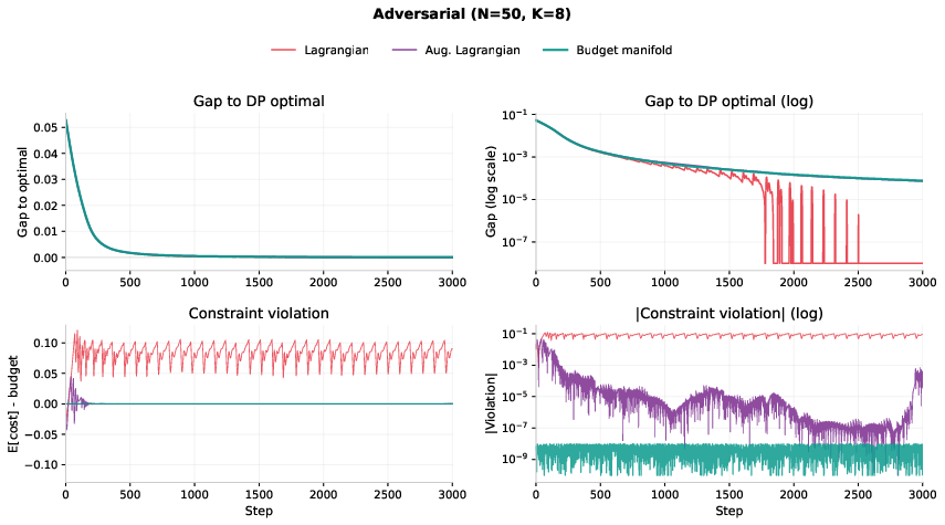
- Lagrangian methods: Techniques that enforce constraints by introducing Lagrange multipliers into the objective. "On hard instances, as we show in Section~\ref{sec:mckp}, Lagrangian methods oscillate."
- level set: The set of points where a function takes on a constant value. "Therefore, by the regular value theorem, the level set is a smooth -dimensional Riemannian submanifold of ."
- MILP: Mixed-Integer Linear Programming, where some variables are constrained to be integer while others are continuous in a linear optimization problem. "IMPQ~\citep{zhao2025impq} (Shapley-based surrogate with pairwise layer interactions, solved via MILP)"
- momentum transport: Moving optimizer momentum vectors from one tangent space to another after retraction on a manifold. "we propose Riemannian Constrained Optimization (RCO), which wraps tangent projection, binary-search retraction, and momentum transport around a standard Adam step."
- monotonic retraction: A retraction whose target function varies monotonically with the retraction parameter, enabling efficient root finding. "The closed-form derivative~\eqref{eq:retraction_deriv} also enables Newton retraction in 2--3 iterations; we use binary search for simplicity, but the multi-constraint extension... builds on Newton root-finding using the same derivative." (See Proposition title: "Monotonic retraction")
- multiple-choice knapsack problem (MCKP): A combinatorial optimization problem where exactly one item must be chosen from each group to maximize utility under a budget. "The multiple-choice knapsack problem (MCKP) admits closed-form gradients and an exact DP solution"
- Newton retraction: A retraction method using Newton’s method to solve for the retraction parameter using derivative information. "The closed-form derivative~\eqref{eq:retraction_deriv} also enables Newton retraction in 2--3 iterations"
- regular value theorem: A result ensuring that preimages of regular values are smooth submanifolds. "Therefore, by the regular value theorem, the level set is a smooth -dimensional Riemannian submanifold of ."
- retraction: In Riemannian optimization, a map that brings an off-manifold point back onto the manifold along a feasible path. "Optimizing on a manifold requires three operations: tangent projection (restricting gradients to the tangent plane), retraction (mapping an iterate that has drifted off the surface back onto it), and vector transport"
- Riemannian gradient: The gradient vector field defined with respect to the manifold’s metric, i.e., projected onto the tangent space. "we verify in the appendix that... the projected gradient recovers the Riemannian gradient"
- Riemannian manifold: A smooth manifold equipped with an inner product (metric) on each tangent space, enabling geometric notions like lengths and angles. "we observe that under softmax relaxation, the budget constraint defines a smooth Riemannian manifold in logit space"
- Sinkhorn projections: Iterative normalization procedures to project matrices onto the set of doubly stochastic matrices. "doubly stochastic matrices require iterative Sinkhorn projections~\citep{douik2019manifold}"
- slack variable: An auxiliary variable that converts an inequality constraint into an equality by absorbing excess budget. "A slack variable with extends the manifold to inequality constraints"
- softmax Jacobian: The matrix of derivatives of the softmax function, characterizing how logits perturbations change probabilities. "the softmax Jacobian interacting with linear cost gives the level set a ``clean'' geometry."
- Stiefel manifold: The set of matrices with orthonormal columns; common constraint set in optimization. "By comparison, retraction on the Stiefel manifold requires QR or polar decomposition"
- straight-through estimator (STE): A gradient estimator that bypasses non-differentiable operations by using surrogate gradients. "the STE~\citep{bengio2013estimating} replaces the non-differentiable with soft probabilities"
- tangent plane: The linear space of directions tangent to a manifold at a point. "At each point, the tangent plane is the subspace of directions tangent to the surface"
- tangent projection: Projecting a vector (e.g., a gradient) onto the manifold’s tangent space to respect constraints. "Optimizing on a manifold requires three operations: tangent projection (restricting gradients to the tangent plane), retraction..., and vector transport"
- vector transport: A rule to move tangent vectors from one point’s tangent space to another’s on a manifold. "vector transport (moving vectors such as optimizer momentum from one tangent plane to another as the iterate moves along the surface)"
Collections
Sign up for free to add this paper to one or more collections.

