An Explicit Solution to Black-Scholes Implied Volatility
Abstract: This paper identifies what appears to be the first explicit formula for Black-Scholes implied volatility, resolving a 50-year-old problem in option pricing. The key observation is that the call price can be written as a survival probability of an inverse Gaussian distribution. Inverting this identity expresses implied volatility directly through the corresponding quantile function. The formula uses only observable option inputs and requires no initial guess, iterative inversion, approximation, asymptotic expansion, or infinite series. Numerical tests recover implied volatility to machine precision and show the formula to be about 3.4 times faster than a current state-of-the-art reference benchmark.
Paper Prompts
Sign up for free to create and run prompts on this paper using GPT-5.
Top Community Prompts
Explain it Like I'm 14
A Simple Explanation of “An Explicit Solution to Black–Scholes Implied Volatility”
Overview: What is this paper about?
This paper is about a big problem in options trading: turning an option’s market price into its “implied volatility.” Traders use implied volatility as a quick way to describe how “bouncy” (risky) they think a stock or index will be in the future. The Black–Scholes formula easily goes from volatility to price, but going backwards—from price to implied volatility—has been tricky for 50 years and usually needs trial-and-error methods. This paper claims to give the first exact, direct formula to get implied volatility from the option price—no guesswork, no iteration.
What questions is the paper trying to answer?
- Can we write a clean, one-step formula that turns a call (or put) option price into its Black–Scholes implied volatility?
- Can this formula be both exact (no approximation) and fast to compute?
- Can we give a simple probability meaning to implied volatility, not just see it as the output of a numerical solver?
How did the author do it? (Methods in everyday language)
The key idea is to look at the Black–Scholes call price in a new way: as a probability.
- Think of a “random walker” (like a person taking random steps) trying to reach a gate. How long it takes to reach the gate is a random time. Mathematicians know that the distribution of those “first times to reach a level” often follows something called an inverse Gaussian distribution.
- The author shows that the Black–Scholes call price can be written as a survival probability for that inverse Gaussian distribution. “Survival probability” just means “the chance that the random walker has not reached the gate yet by a certain time.”
- Once the call price is turned into a probability, you can invert it using the distribution’s “quantile function.” A quantile is like asking, “What height marks the tallest 30% of people?” In statistics software, quantile functions are standard tools that turn a probability into the corresponding “cutoff value.”
Putting this together:
- Convert the observed option price into a probability level on the inverse Gaussian scale.
- Use the inverse Gaussian quantile to flip that probability into a number.
- Translate that number into implied volatility with a simple final step.
For the special case when the strike equals the forward price (“at-the-money”), the formula becomes even simpler and uses the normal distribution’s quantile (another standard function).
The author also uses put–call parity (a standard relation between call and put prices) to write a similar one-step formula for put options.
What did the paper find, and why does it matter?
Main findings:
- A direct, explicit formula: The paper presents a closed-form expression that gives Black–Scholes implied volatility from an option’s market price using only standard inputs (price, strike, time to maturity, etc.) and one special but standard function (the inverse Gaussian quantile), which is available in common math libraries.
- No iteration or initial guess: Unlike traditional methods that repeatedly “guess and check,” this formula computes implied volatility in one shot.
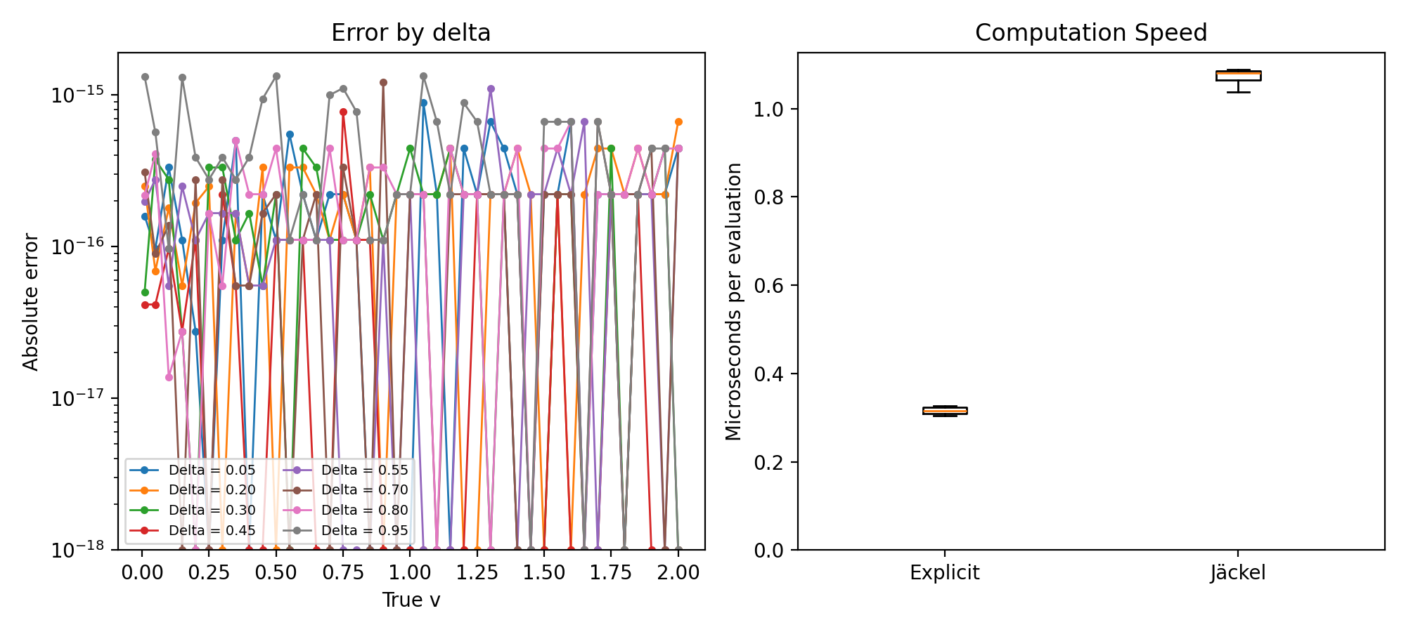
- Exactness and speed: In tests covering a wide range of cases, the formula recovers the true implied volatility to machine precision (tiny errors near 10-16) and runs about 3.4 times faster than a widely respected benchmark algorithm (“Let’s Be Rational” by Jäckel).
Why this matters:
- Markets quote and compare options by implied volatility all day, every day. A faster, exact method can make option pricing, risk management, and model calibration more efficient and more reliable.
- It gives a new way to “think” about implied volatility: not as the end result of a search, but as a direct probability-to-quantile conversion. In other words, the option price picks a probability level, and the implied volatility is the matching quantile on a specific probability scale.
What does this mean going forward? (Impact and implications)
- Practical impact: Trading systems, risk tools, and research software can compute implied volatility faster and with guaranteed accuracy—helpful anywhere large numbers of options are processed (like in real-time trading or backtesting).
- Conceptual clarity: The result reframes implied volatility as a “distributional transform” of price—connecting it to the chance that a random, drifting walk hasn’t hit a target by a certain “variance time.” This may inspire new ways to analyze and visualize volatility surfaces or to teach the subject.
- Broader research: The success here might motivate similar approaches in more advanced models beyond Black–Scholes, or lead to new probabilistic insights in option pricing.
Quick glossary (helpful terms)
- Option (call): A contract that gives you the right (not the obligation) to buy an asset at a fixed price (the strike) by a certain date.
- Strike price (K): The price at which the option lets you buy (call) or sell (put) the asset.
- Implied volatility (IV): The market’s “best guess” of future volatility, extracted from option prices.
- Black–Scholes formula: A classic formula that computes an option’s price from inputs like current price, strike, time, and volatility.
- Quantile function: A standard math tool that turns a probability (like 0.8) into the value where 80% of outcomes lie below it.
- Inverse Gaussian distribution: A probability model often used for “time to reach a target” under random movement with drift. Here, it’s the bridge between price and implied volatility.
In short, this paper claims to solve a long-standing problem by showing that implied volatility isn’t something you have to search for—it’s something you can calculate directly, quickly, and exactly, by reading the right quantile off the right probability scale.
Knowledge Gaps
Knowledge gaps, limitations, and open questions
Below is a concise list of unresolved issues and concrete research directions suggested by the paper.
Mathematical foundations and rigor
- Provide a complete, rigorous proof that the normalized Black–Scholes call price equals the inverse-Gaussian survival function for all admissible inputs, including a careful reconciliation of parameterizations and correction of apparent typesetting errors in the stated survival function (Eq. (3)).
- Prove monotonicity, injectivity, and global well-posedness of the proposed inversion map σ(K, C) for all arbitrage-admissible prices, including continuity and differentiability across the k → 0 boundary and verification that the ATM formula is the correct limit of the k ≠ 0 expression.
- Characterize the analytic class of the new “explicit” function (in terms of special functions) and reconcile it formally with Gerhold (2012)’s non D-finite result, clarifying what types of closed forms remain ruled in or out.
- Derive precise asymptotics of σ(K, C) as c → 0+, c → 1−, k → ±∞, v → 0+, and v → ∞, and connect these to known implied-vol asymptotics for consistency checks and for building numerically stable tail treatments.
Domain, inputs, and financial admissibility
- Specify the exact admissible domain of inputs (C, K, F, D, T) under no-arbitrage, and develop robust procedures (e.g., projections/clipping) for handling market prices that violate these bounds due to bid–ask spreads, latency, or rounding, including how such adjustments propagate through the quantile transform.
- Clarify treatment of dividends and forwards in settings with discrete dividends or negative interest rates; provide guidance on constructing F from S in such markets and state any constraints required by the formula.
Numerical stability and performance
- Systematically assess the numerical robustness of the inverse-Gaussian quantile evaluation across libraries, parameterizations, and precisions (float32/float64/decimal), including extreme probability arguments near 0 and 1; provide a comprehensive test suite and reference tolerances.
- Develop switching criteria and error bounds for the ATM neighborhood (k ≈ 0), including a principled threshold between the general and ATM formulas and continuity/error guarantees at the switch.
- Design tail-stable computational paths (e.g., asymptotic expansions or reparameterizations) for the inverse-Gaussian quantile when (1 − c)/m is extremely close to 0 or 1, to prevent loss of significance and quantile algorithm failures.
- Benchmark performance beyond scalar CPU tests: vectorized/SIMD execution, multithreaded workloads, GPU acceleration, and low-latency settings; compare against a broader set of solvers (Halley/Householder variants, rational approximations, specialized Newton seeds).
- Investigate custom approximations or tabulations for the specific IG quantile family λ = 1, μ = 2/|k| to reduce latency further while maintaining machine-precision recovery guarantees.
- Provide a detailed ULP-level error analysis for σ recovery and quantify how quantile evaluation error translates to implied-volatility error across the state space.
Empirical validation on real markets
- Validate the method on large, real-world datasets spanning asset classes (equities, FX, rates, commodities), maturities, and moneyness regimes, including deep ITM/OTM, near-expiry options, and ultra-long maturities; report failure modes, convergence issues, and runtime distributions in production conditions.
- Quantify robustness under market microstructure noise, stale quotes, and rounding; provide procedures for propagating price uncertainty to implied-volatility uncertainty via the quantile derivative.
- Extend the numerical evaluation to puts (the paper provides the formula but not empirical tests) and to jointly testing call–put parity consistency under noisy inputs.
Practical implementation and reproducibility
- Release a cross-language, open-source reference implementation (C/C++/Rust/Fortran/Julia/Python) with harmonized inverse-Gaussian parameterization, thorough tests, and reproducible benchmarks; document differences across statistical libraries’ IG parameterizations and quantile algorithms.
- Specify exception-handling strategies (e.g., fallback approximations, safeguarded asymptotics) when the quantile routine returns NaN/Inf or fails to converge, and quantify the impact on accuracy and speed.
- Provide guidance for integration into large-scale IV-surface engines (batch processing, caching, mixed-precision, vectorized kernels), including performance/accuracy trade-offs and memory–latency considerations.
Extensions and further theory
- Derive closed-form expressions (or stable computational formulas) for the derivatives of σ with respect to inputs (dσ/dC, dσ/dK, dσ/dT, dσ/dF, and higher-order terms) by differentiating through the inverse-Gaussian quantile; validate their accuracy and stability for calibration and risk.
- Explore whether analogous explicit inversions exist for other models (e.g., Bachelier/normal, displaced-diffusion, CEV) via alternative distributional transforms and quantiles; delineate the scope of this approach.
- Investigate applications of the variance-space probabilistic interpretation for arbitrage-free surface construction and regularization (e.g., constraints in the GIG/IG quantile domain), and study its implications for SVI or other surface parameterizations.
- Use the GIG representation to develop statistical inference and uncertainty-quantification tools for implied volatility under price noise (e.g., confidence intervals for σ via delta-method with quantile derivatives).
- Analyze computational complexity formally (including constant factors) of the proposed method versus iterative solvers under realistic workload assumptions and quantify when each approach is preferable.
Practical Applications
Immediate Applications
The paper’s explicit inverse-Black–Scholes formula (via inverse Gaussian quantiles) replaces iterative root-finding with a single closed-form evaluation, enabling the following deployable use cases:
- High-throughput implied-volatility engines for trading and market making
- Sectors: Finance, High-frequency trading, Market data
- Tools/products/workflows: Drop-in replacement for “Let’s Be Rational” in C++/Java/Python/R libraries; exchange/order-book IV computation; low-latency quoting and hedging engines
- Assumptions/dependencies: Availability of a robust inverse Gaussian (IG) quantile; correct handling of at-the-forward case (normal quantile); Black–Scholes (BS) convention (positive forward, proper discounting); numerical stability for deep OTM/ITM and extreme maturities
- Real-time volatility-surface construction and calibration
- Sectors: Finance (sell-side/prop), Risk analytics, Market data vendors
- Tools/products/workflows: Faster calibration of SVI/parametric surfaces; denser grids across strikes/maturities; more frequent surface refresh
- Assumptions/dependencies: BS-consistent inputs (C, K, F, D, T); reliable normalization to c and k; IG quantile accuracy in tails
- Massive-scale backtesting and empirical asset pricing
- Sectors: Academia, Quant research, Asset management
- Tools/products/workflows: Reproducible IV labels without initial-guess/tolerance artifacts; shorter runtimes for studies with billions of options
- Assumptions/dependencies: Data cleaning to valid price bounds; consistent forward/discount conventions across datasets
- Risk and XVA platforms leveraging IV for proxies and scenario analyses
- Sectors: Finance (risk management, treasury), Clearing houses
- Tools/products/workflows: Faster IV extraction for VaR/stress pipelines; improved overnight batch throughput and SLA compliance
- Assumptions/dependencies: Continued reliance on BS-IV as a reporting/aggregation coordinate even when pricing models differ
- On-device and in-browser option calculators (retail and professional)
- Sectors: Fintech, Education
- Tools/products/workflows: Mobile/web apps using a single quantile call; no iterative loops; better battery and latency profiles
- Assumptions/dependencies: JS/WebAssembly/Rust/C++ implementations of IG quantile; ATM branch uses normal quantile
- Smart contracts and on-chain IV oracles (gas/cost-sensitive computation)
- Sectors: DeFi, Blockchain oracles
- Tools/products/workflows: Solidity/Rust/Cairo libraries implementing the closed form; reduced gas vs iterative solvers; deterministic results
- Assumptions/dependencies: Efficient fixed-point approximations or precompiled IG quantile; careful tail handling; BS framework applicability to on-chain option designs
- Education and training (conceptual clarity and pedagogy)
- Sectors: Academia, Professional certifications (CFA/FRM), Corporate training
- Tools/products/workflows: Teaching IV as a direct distributional transform; variance-space probability interpretation; problem sets without numerical root-finding
- Assumptions/dependencies: Students’ access to statistical libraries; alignment with BS conventions
- Data-quality diagnostics and sanity checks
- Sectors: Market data operations, Compliance, Audit
- Tools/products/workflows: Immediate IV failure modes flag out-of-range prices (e.g., arbitrage violations); deterministic mapping simplifies QA
- Assumptions/dependencies: Proper treatment of put–call parity and forward estimation; bounds checks on normalized c and k
- Differentiable analytics pipelines
- Sectors: Quant ML/AI, Portfolio optimization
- Tools/products/workflows: Autograd/AD-friendly IV layer (no non-smooth solver iterations); cleaner gradients for surface fitting and operator-learning models
- Assumptions/dependencies: Availability of IG quantile derivatives or AD-capable implementation; numerical stability near ATM and tails
- Cloud cost and energy usage reductions
- Sectors: Cloud-native analytics, ESG/Green IT
- Tools/products/workflows: Lower CPU cycles per IV; scale-down compute clusters for real-time analytics
- Assumptions/dependencies: Reliable vectorized implementation (SIMD/GPU where applicable); profiling confirms 3.4× speedup holds in production data distributions
Long-Term Applications
The new representation (price as an inverse Gaussian survival probability; IV as the corresponding quantile) suggests broader developments that require further research, scaling, or standardization:
- Exchange and regulatory standardization of implied-volatility reporting
- Sectors: Exchanges, Regulators, Market data vendors
- Tools/products/workflows: Official IV definition via explicit closed form; harmonized benchmarks for best-execution and transaction cost analysis
- Assumptions/dependencies: Industry consensus-building; validation under diverse market conventions (dividends, forwards, discrete rates)
- Hardware acceleration and specialized kernels
- Sectors: Low-latency trading, HPC
- Tools/products/workflows: FPGA/ASIC/AVX-optimized IG quantile; microcode or math-library primitives for IG inverse CDF
- Assumptions/dependencies: Stable parameterization across devices; thorough testing for tails and denormals
- Quantile-based surface diagnostics and arbitrage detection
- Sectors: Risk, Market surveillance
- Tools/products/workflows: Variance-space probability thresholds for outlier detection; real-time flags for crossed surfaces or stale quotes
- Assumptions/dependencies: Research on thresholds and statistical power; integration with existing no-arbitrage checks and SVI constraints
- Extensions to other models and payoffs (inspired by the first-passage link)
- Sectors: Quant research, Derivatives engineering
- Tools/products/workflows: Investigate analogous explicit inverses for Bachelier (normal) IV, displaced-diffusion, or certain exotics (barriers) using FPT distributions
- Assumptions/dependencies: Existence of similar survival–price identities; tractable inverse quantiles; rigorous error controls where exactness is not attainable
- Robust extreme-tail computation standards
- Sectors: Risk, Vendor libraries
- Tools/products/workflows: High-precision IG quantile for ultra-long maturities/deep strikes; interval arithmetic/fallback asymptotics
- Assumptions/dependencies: Community-maintained test suites and reference datasets; mixed-precision strategies for edge cases
- Integrated “exact IV” microservices and APIs
- Sectors: Fintech, Enterprise analytics
- Tools/products/workflows: Centralized services offering BS IV with SLAs, versioning, and audit trails; plugin modules for Excel, MATLAB, Python, R, Julia
- Assumptions/dependencies: Security, latency budgets, and high-availability infrastructure; clear parameterization mapping to client libraries
- ML architectures leveraging the explicit IV as a differentiable operator
- Sectors: AI in finance
- Tools/products/workflows: Incorporate the IG-quantile-based IV as a layer in deep smoothing/operator-learning for surfaces; end-to-end training with consistent IV targets
- Assumptions/dependencies: Stable gradients of IG quantile; regularization for tail regimes; empirical validation against iterative baselines
- Broader economic studies and policy analyses using consistent IVs at scale
- Sectors: Academia, Policy institutions
- Tools/products/workflows: Large cross-asset/cross-market studies of volatility premia and risk-transfer with uniform IV computations; policy stress tests using standardized IVs
- Assumptions/dependencies: Data harmonization across venues; alignment on forward/discount conventions; documented methodology for replication
Notes on implementation dependencies and scope:
- Parameterization care: Library “inverse Gaussian” parameterizations vary. Map the paper’s IG(mean=μ, shape=λ) to the target library (e.g., SciPy’s invgauss uses a different convention with scale). Verify against unit tests, especially the ATM branch that uses the normal quantile.
- Domain limits: The formula presumes positive forwards (log-moneyness well-defined). For assets or rates modeled with potentially negative forwards (e.g., some IR contexts), BS is not appropriate; use Bachelier IV instead.
- Numerical stability: Use the provided ATM formula near k≈0; apply safeguards for c close to 0 or 1 (deep OTM/ITM) and very small/large T.
- Market realism: While markets are not BS, BS-implied volatility is the common quoting coordinate across models. These applications rely on that convention, not on BS being the true data-generating process.
Glossary
- Asymptotic expansion: An approximation of a function by a series that becomes increasingly accurate in a limit (e.g., large or small parameter). "requires no initial guess, iterative inversion, approximation, asymptotic expansion, or infinite series."
- At-the-forward (strike): The special case where the strike equals the forward price, simplifying certain option pricing expressions. "for the at-the-forward strike level."
- Black--Scholes formula: The closed-form option pricing model assuming lognormal underlying dynamics with constant volatility and rates. "The Black--Scholes formula is explicit from volatility to option price."
- Brownian motion: A continuous-time stochastic process with independent, normally distributed increments used to model random movement. "Let denote standard Brownian motion"
- Call delta (Delta): The sensitivity of a call option’s price to changes in the underlying asset’s price. "call delta is set to "
- Change of measure: A probabilistic technique that switches the underlying probability measure to simplify expectations or probabilities. "under a suitable change of measure."
- D-finite: A class of functions that satisfy a linear differential equation with polynomial coefficients. "implied volatility is not -finite"
- Diffusion volatility: The instantaneous volatility parameter in a diffusion (continuous-time) stochastic process. "diffusion volatility $1$"
- First-passage time: The random time at which a stochastic process first reaches a specified level. "first-passage-time interpretation."
- Forward (price): The current price for future delivery of an asset, often denoted by in option pricing. "strike , forward , risk-free discount factor "
- Generalized inverse Gaussian distribution (GIG): A three-parameter family of continuous probability distributions that generalizes the inverse Gaussian. "where denotes the generalized inverse Gaussian distribution"
- Implied variance: The square of implied volatility (), representing the variance implied by option prices. "the probability that implied variance clears this moneyness-induced barrier."
- Implied volatility: The volatility value that, when input into a pricing model like Black–Scholes, reproduces the observed option price. "explicit formula for Black--Scholes implied volatility"
- In-the-money (ITM): An option with positive intrinsic value (for calls, when spot/forward exceeds strike). "the call is in the money."
- Inverse Gaussian distribution: A two-parameter continuous distribution often associated with first-passage times of Brownian motion with drift. "survival probability of an inverse Gaussian distribution."
- Inverse Gaussian quantile function: The inverse of the inverse Gaussian cumulative distribution function, mapping probabilities to quantiles. "the only non-elementary operation is the inverse Gaussian quantile function "
- Log-moneyness: The logarithm of the ratio of strike to forward (or spot), a normalized measure of moneyness. "where is the normalized call price and is forward log-moneyness."
- Machine precision: The smallest difference detectable by a given floating-point representation, typically double precision in numerical work. "recover implied volatility to machine precision"
- Moneyness: A dimensionless measure comparing the underlying price to the strike, indicating ITM/ATM/OTM status. "a moneyness-specific variance scale."
- Normalized call price: A call price scaled by discount and forward to remove units, often simplifying formulas. "The normalized Black--Scholes European call price is"
- Out-of-the-money (OTM): An option with zero intrinsic value (for calls, when strike exceeds spot/forward). "First take an out-of-the-money call"
- Put--call parity: A no-arbitrage relationship linking prices of European calls and puts with the same strike and maturity. "The corresponding put formula follows from the put--call parity"
- Quantile function: The inverse of a cumulative distribution function, mapping probabilities to values. "expresses implied volatility directly through the corresponding quantile function."
- Risk-free discount factor: The present value factor for a future payoff discounted at the risk-free rate. "risk-free discount factor "
- Survival function: One minus the cumulative distribution function, giving the probability of exceeding a threshold. "Its survival function is"
- Total implied volatility: The product of volatility and square root of time (), often used as a single scale parameter. "Let be the total implied volatility."
- Variance space: A perspective where quantities are parameterized by variance rather than returns or time. "moves the probability statement into variance space."
- Volatility risk premia: The compensation investors demand for bearing volatility risk, inferred from option prices. "tests of volatility risk premia."
- Volatility surface: A function describing implied volatility across strikes and maturities for an underlying. "volatility-surface modelling"
Collections
Sign up for free to add this paper to one or more collections.