Implicit Velocity Correction Schemes for Scale-Resolving Simulations of Incompressible Flow: Stability, Accuracy, and Performance

Abstract: Scale-resolving simulations of high Reynolds number incompressible flows are often limited by the Courant-Friedrichs-Lewy (CFL) stability restriction imposed by explicit time-stepping schemes, resulting in small time step sizes and long time-to-solution. In this work, we systematically compare two implicit formulations of the velocity correction scheme -- a linear-implicit approach and a sub-stepping (or semi-Lagrangian) method -- against a standard semi-implicit formulation within a high-order spectral/hp element framework. The schemes are assessed in terms of stability limits, temporal accuracy, and computational performance for implicit large-eddy simulation of the Imperial Front Wing benchmark, a complex high Reynolds number geometry with curved surfaces that imposes strict CFL constraints. Both implicit schemes extend the stability limit by up to two orders of magnitude in time step size. While increasing the cost per time step, they reduce the overall time-to-solution by up to a factor of eleven. Accuracy analysis shows that time step sizes up to twenty times larger than the explicit limit have only minor impact on resolving laminar-turbulent transition and key flow statistics. The results quantify the trade-off between stability, accuracy, and computational cost for implicit velocity correction schemes on complex geometries and provide guidance for selecting time integration strategies in large-scale scale-resolving simulations.

• The paper demonstrates that both implicit schemes extend the permissible time step by up to two orders of magnitude relative to the semi-implicit baseline.
• The paper introduces a sub-stepping semi-Lagrangian method and a linear-implicit approach, analyzing their trade-offs in stability, accuracy, and computational cost.
• The paper concludes that adaptive implicit strategies are essential to balance speed and physical fidelity in wall-resolved LES of complex geometries.

Implicit Velocity Correction Schemes in Scale-Resolving Incompressible Flow Simulation

Introduction

The paper "Implicit Velocity Correction Schemes for Scale-Resolving Simulations of Incompressible Flow: Stability, Accuracy, and Performance" (2604.16057) provides a comprehensive examination of two implicit time-integration variants for velocity correction schemes—specifically, a linear-implicit approach and an advection sub-stepping (semi-Lagrangian/OIFS) scheme—within the context of high-order spectral/hp element wall-resolved large-eddy simulation (WRLES) of incompressible flow around a complex, high Reynolds number multi-element wing geometry. The authors analyze the trade-offs in stability, accuracy, and performance relative to a standard semi-implicit IMEX velocity-correction baseline. This study isolates the influence of the temporal integration by keeping all other numerical and physical parameters fixed, using the extruded Imperial Front Wing (eIFW) configuration as a reference case.

Numerical Methodology and Algorithmic Design

The work leverages the velocity correction fractional step method—a prevailing approach in large-scale incompressible flow solvers based on operator splitting of the Navier–Stokes equations into pressure Poisson and velocity subproblems [Karniadakis1991, Guermond2003], facilitated here by the high-order Nektar++ framework [Cantwell2015, Moxey2020].

• Semi-implicit Formulation: Employs explicit advection (Eulerian frame) and implicit diffusion, resulting in a classical IMEX splitting. This method is constrained by the global Courant–Friedrichs–Lewy (CFL) condition due to explicit advection.
• Sub-stepping Scheme: Augments each physical time step with multiple explicit pseudo-time advection solves (in a semi-Lagrangian/OIFS fashion), significantly relaxing the stability restriction while retaining linear system structure for pressure/diffusion (see Figure 1).

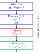
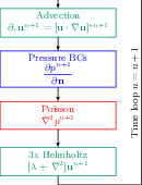
Figure 1: Semi-implicit scheme.

• Linear-implicit Scheme: Linearizes the advection operator at each step, solving an ADR (Advection-Diffusion-Reaction) system. This introduces a time-dependent nonsymmetric matrix but avoids nonlinear solves.

All approaches are realized within a high-order, boundary-conforming spectral/hp element discretization, incorporating static condensation for efficient solution of linear systems and aggressive over-integration/SVV for robustness at high Reynolds numbers (see Figure 2).

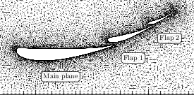
Figure 2: A cross-section of the near field mesh highlighting the fine boundary layer mesh on the wing elements and floor.

Benchmark Configuration: Wall-Resolved LES on the eIFW Geometry

The eIFW benchmark is the most stringent publicly available wall-resolved, ground-effect multi-element wing configuration, characterized by intricate transition dynamics, boundary layer separation, and strong geometric restrictions on the local time step due to mesh clustering near walls (see Figure 3; mesh statistics, Figure 4).

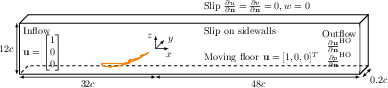
Figure 3: Computational domain and boundary conditions with wing elements. Note that the wing elements are enlarged by factor 4 for visibility.

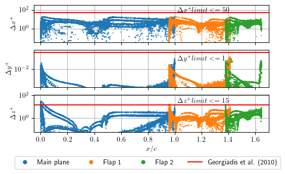
Figure 4: Distribution of wall units $\Delta x^+, \Delta y^+, \Delta z^+$ for the time-averaged flow field on all wing elements. Note that $\Delta y^+$ is the wall-normal direction.

Mesh design employs high-order curved elements with Taylor–Hood approximation ($P_v=4, P_p=3$), providing $\mathcal{O}(10^7)$ global DOF and stringent clustering in wall-parallel directions for accurate boundary layer capture.

Stability Analysis

A primary finding is that both implicit methods (sub-stepping and linear-implicit) extend the admissible time step by up to two orders of magnitude relative to the semi-implicit baseline. Specifically, CFL stability boundaries increase from $\mathcal{O}(1)$ (semi-implicit) to $\mathcal{O}(10^2)$ (implicit), demonstrating near-linear scaling of attainable CFL number with physical time step for stable and physically consistent solutions (see Figures 9 and 10).

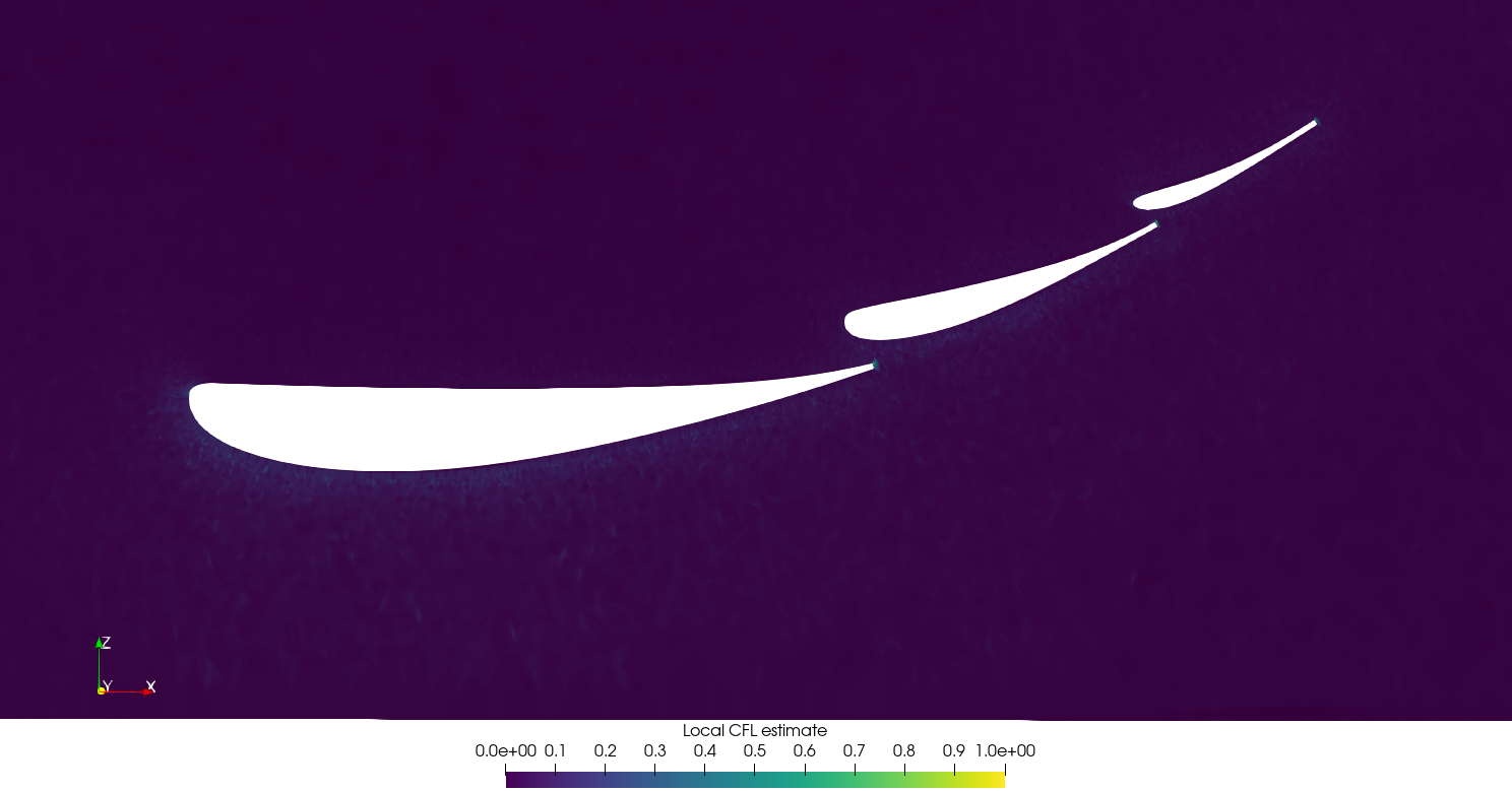
Figure 5: Time-averaged CFL estimate for the mid-plane and semi-implicit scheme with given time step.

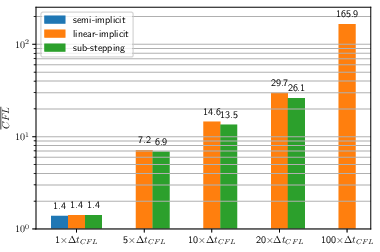
Figure 6: Time-average of the maximum local CFL estimate for all schemes at increasing time step size.

The linear-implicit approach further allows especially large time steps under an equal-order $(P_v = P_p)$ discretization without loss of stability.

Accuracy and Physical Fidelity

Across all schemes, at the semi-implicit reference time step, predictions for time-averaged aerodynamic coefficients, transition locations, and wall-resolved spectra are nearly indistinguishable (see Figures 5–8, 11–16). Statistical and spectral comparisons confirm full resolution of transition dynamics and turbulent statistics up to Strouhal $St\sim 10^2$.

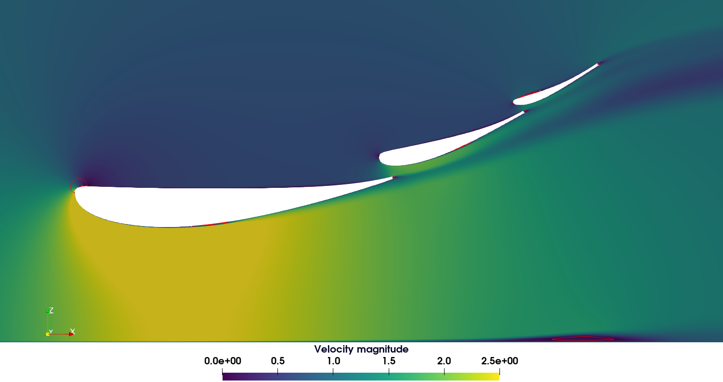
Figure 7: Time-averaged velocity magnitude at the midplane ($y=0.1c$). Recirculation regions are highlighted in red as contours of zero streamwise velocity $u = 0$.

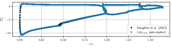
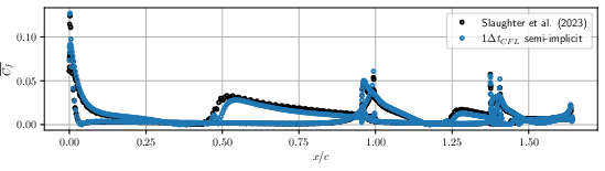*Figure 8: Pressure coefficient $\Delta y^+$0. *

Increasing the time step size for the implicit schemes results in a gradual degradation in transition-sensitive surface metrics (upstream shift in the location of laminar separation bubble and altered skin-friction distribution; Figures 14, 17, 25), while global forces and low-frequency spectra are comparatively robust (Figures 13, 16, 18). At very large time steps ($\Delta y^+$1 explicit units), the resolved physics is no longer trustworthy: transition mechanisms and spectral content are fundamentally altered, especially in high-frequency regimes.

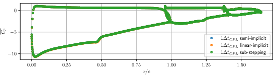
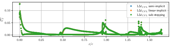
Figure 9: Pressure coefficient $\Delta y^+$2.

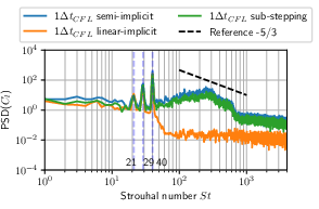
Figure 10: Power spectral density of the lift coefficient summed over all wing elements. Comparison of the influence of the time-stepping scheme with time step size.

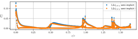
Figure 11: Time-averaged skin-friction coefficients comparing the influence of Reynolds number. Data are averaged in the spanwise direction.

Performance and Scalability

The performance landscape is strongly influenced by the per-step computational overhead introduced by the implicit schemes:

• Sub-stepping: Overhead scales with the number of advection sub-steps. While cost per step is significantly higher, the overall time-to-solution can be up to $\Delta y^+$3 faster at stability-maximal step sizes, but is limited by increased pressure system conditioning and pseudo-time cost at very large steps (see Figures 19–22).
• Linear-implicit: Per-step overhead is more severe (matrix assembly, GMRES cycling), but the method achieves the largest overall speedup—over $\Delta y^+$4 faster than baseline for the largest stable step, provided that the physical accuracy requirements are met.

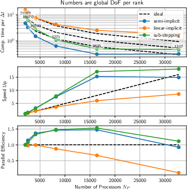
  Figure 12: Strong scaling of the semi-implicit, sub-stepping, and linear-implicit schemes in terms of average time per time step, speed-up, and parallel efficiency.

  

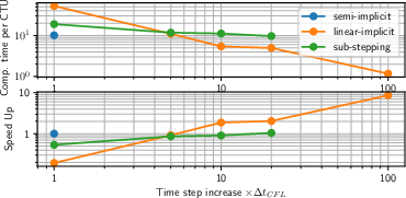
  Figure 13: Reduction in time-to-solution relative to the semi-implicit reference as a function of time step size for the sub-stepping and linear-implicit schemes.

For both schemes, the break-even point (where speed benefit outweighs per-step cost) occurs at a moderate step size increase ($\Delta y^+$5–$\Delta y^+$6), beyond which further speedup is incremental due to the increasing iteration count of Krylov solvers for the stiffest systems.

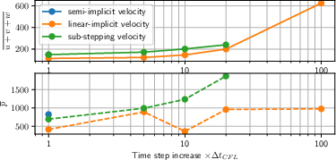
Figure 14: Average iteration counts for the pressure solve and the sum of the three velocity solves as a function of time step size.

Implications and Future Directions

This systematic study quantifies, for the first time in a complex, statistically converged industrial WRLES setting, the precise trade-off envelope between stability, accuracy, and computational cost across a set of linearly implicit velocity correction variants. The results provide concrete guidance for the selection of time integration schemes:

• Transient phases or initial state spin-up: Large step, implicit schemes (especially linear-implicit) can dramatically accelerate the route to statistical stationarity, provided transition and high-frequency details are not essential.
• Statistical sampling or when accurate transition dynamics are required: Step sizes should remain within $\Delta y^+$7–$\Delta y^+$8 times the explicit limit for sub-stepping, and lower still for linear-implicit, to avoid systematic errors in wall/boundary layer quantities.
• Long, stationary averaging: Semi-implicit or moderately implicit approaches remain preferable for maximizing accuracy per computational cost.

Potential future advances include coupling matrix-free linear-implicit velocity operators (to reduce assembly cost), optimized preconditioning tailored for large CFL regimes, and adaptivity in time step size—using implicit steps for transient, error-tolerant phases and reverting to explicit/semi-implicit for detail-resolving phases.

Conclusion

The paper decisively establishes that implicit velocity correction schemes can offer significant reductions in time-to-solution for scale-resolving incompressible flow simulation on complex geometries, but only when the increased permissible time step does not violate physically required temporal resolution. The stability advantage of implicit schemes must be balanced against computational cost escalation and accuracy loss from excessive step size. Practical deployment of these methods should exploit adaptive strategies which match the degree of implicitness and step size to the actual error tolerance required by the physical phase of the simulation. The methodology and findings constitute a roadmap for further development and industrial application of advanced high-order incompressible LES solvers targeting large-scale, wall-resolved turbulent flows.