A short proof of near-linear convergence of adaptive gradient descent under fourth-order growth and convexity
Abstract: Davis, Drusvyatskiy, and Jiang showed that gradient descent with an adaptive stepsize converges locally at a nearly-linear rate for smooth functions that grow at least quartically away from their minimizers. The argument is intricate, relying on monitoring the performance of the algorithm relative to a certain manifold of slow growth -- called the ravine. In this work, we provide a direct Lyapunov-based argument that bypasses these difficulties when the objective is in addition convex and a has a unique minimizer. As a byproduct of the argument, we obtain a more adaptive variant than the original algorithm with encouraging numerical performance.
Paper Prompts
Sign up for free to create and run prompts on this paper using GPT-5.
Top Community Prompts
Explain it Like I'm 14
What is this paper about?
This paper studies how to make gradient descent (a basic method for minimizing a function) work much faster when the function is unusually “flat” near its minimum. In particular, the authors look at smooth convex functions that grow like the fourth power of the distance to the minimum (called fourth-order growth). They give a short, simple proof that a small change to gradient descent—using an adaptive rule to decide when to take a special “Polyak step”—converges very quickly (nearly linearly) once you start close enough to the minimum. They also present a slightly more adaptive version of the algorithm that performs well in experiments.
What questions are they answering?
- If a function is very flat in some directions near its minimum (so regular gradient descent is slow), can a smart choice of step sizes still make the method converge fast?
- Can we prove this fast convergence with a simpler argument than earlier work?
- Can we turn that argument into a practical algorithm that’s easy to run and tune?
How do they approach the problem? (Simple explanations of key ideas)
First, the basics:
- Gradient descent: Imagine standing on a landscape and always stepping downhill in the direction of steepest descent (the gradient). The size of the step is the “stepsize.”
- Convex function: A bowl-shaped landscape; any line between two points on the graph lies above the graph. This rules out bumps and multiple local minima.
- Fourth-order growth: Near the bottom, the function’s height grows like distance4. That means the landscape is very flat compared to the usual “bowl” (which grows like distance2).
- Polyak step: A special step size that uses how high you are (f(x)) and how steep it is (the gradient) to take a single, well-aimed step: step size = (f(x) − best possible value)/||gradient||2.
What makes things tricky?
- Near the minimum, some directions are steep and others are very flat. The usual curvature matrix (the Hessian) is “singular,” meaning it has zero curvature in some directions. Earlier work tracked a curved “path of slow growth” called a ravine. That proof was technical.
What’s the simpler idea here?
- Split movement into two parts: the steep directions (call them P) and the flat directions (call them Q).
- When you take normal gradient steps with a small fixed stepsize, the part of the gradient in the steep directions shrinks at a steady (linear) rate. This pulls you toward a region where the function truly behaves like distance4 (the “fourth-power regime”).
- Once you are in that regime, one Polyak step gives a strong shrink in distance to the minimum.
- Convexity is crucial: it cancels certain “annoying” cubic terms that would otherwise make the geometry twist and be harder to manage. With convexity, the simpler P/Q split works cleanly, so we don’t need to follow the curving ravine.
Turning this into an algorithm:
- Use regular gradient descent with a fixed stepsize most of the time.
- Keep an eye on a simple ratio R(x) = f(x) / ||∇f(x)||4/3. When this ratio is large enough, it signals you are in the fourth-power regime.
- When R(x) crosses a threshold, take one Polyak step. Then go back to gradient steps.
In plain steps:
- Start close to the minimum with a small stepsize.
- Repeat:
- If R(x) is small, take a normal gradient step.
- If R(x) is big, take one Polyak step (a well-aimed long step).
- This combination steadily moves you in and then quickly down.
What did they prove, and why is it important?
Main result (informally):
- Under fourth-order growth, convexity, and a unique minimizer, the proposed adaptive GD–Polyak method converges quickly (nearly linearly) once you are close enough to the minimum.
- “Nearly linear” here means you shrink the error by a constant factor every so many steps, up to some extra logarithmic factors. More precisely, to get within distance ε of the minimum, the number of gradient/function evaluations is on the order of (1/η)·log(1/ε)·log(start_distance/ε), where η is the stepsize.
Why this matters:
- Standard gradient descent can be slow under fourth-order growth (the landscape is very flat).
- The method here only needs simple ingredients (a constant stepsize and an occasional Polyak step) and a straightforward “trigger” (the ratio R(x)).
- The proof is shorter and more transparent than earlier “ravine-tracking” arguments.
Evidence from experiments:
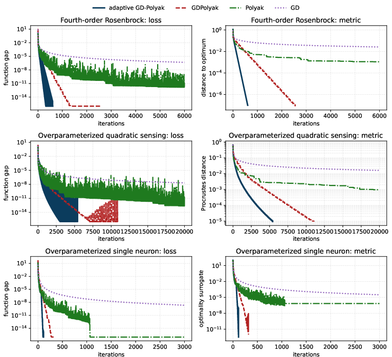
- On several test problems with fourth-order growth (including versions of Rosenbrock, matrix sensing, and a simple neural model), the new method converged much faster than plain gradient descent and matched or beat a prior adaptive scheme—all with simple tuning.
What’s the impact going forward?
- Practical optimization: Many modern models (e.g., over-parameterized matrix factorization or neural nets) create flat directions near solutions. This paper offers a simple, effective way to speed up training in such settings.
- Theory made simpler: The new Lyapunov-style proof (think “a measuring stick that always goes down”) avoids complicated geometric machinery, making the results easier to understand and extend.
- Easy to implement: The algorithm requires only basic quantities (f(x), ∇f(x)), a fixed stepsize, and a simple threshold rule—no heavy extras.
Extra note: What if you don’t know the best possible value f*?
The Polyak step uses f*. In practice, you can start with a safe lower bound (like 0 for nonnegative losses) and refine it over time using the values you observe. The authors outline a simple outer loop that updates this estimate and keeps the convergence guarantees, adding only a small extra logarithmic factor to the total work.
Knowledge Gaps
Below is a concise, actionable list of limitations, knowledge gaps, and open questions that remain after this paper. These items focus on what is missing, uncertain, or left unexplored, and are phrased to guide future research.
- Global guarantees: The main result is local. It remains open to characterize basins of attraction and give global convergence guarantees (or sufficient conditions ensuring entry into the local neighborhood) for the proposed adaptive GD–Polyak scheme.
- Beyond convexity: The analysis requires convexity near the minimizer. Extending the Lyapunov argument to nonconvex settings—especially when the cubic coupling term does not vanish—remains open.
- Weaker structural assumption: The authors note convexity could be replaced by the condition P∇³f(0)[u,u]=0 for all u∈Null(H), but they do not analyze this formally. Provide a complete theory under this weaker, verifiable hypothesis and identify broad function classes where it holds.
- Multiple/Non-isolated minimizers: The proof assumes an isolated (unique) minimizer. Extending the result to problems with a manifold of minimizers (or more general solution sets) is unresolved.
- Degenerate Hessian edge case (H=0): The analysis assumes a nonzero singular Hessian with range(P)≠{0}. The purely quartic case with H=0 (hence P={0}) is not treated; convergence behavior and algorithmic adjustments for this edge case are open.
- Rate optimality: The established complexity O(η⁻¹ log(1/ε)·log(x₀/ε)) has an extra logarithmic factor. It is open whether this can be removed (e.g., to O(η⁻¹ log(1/ε))) or whether the double-log factor is information-theoretically necessary under fourth-order growth.
- Parameter selection without hidden constants: The theoretical choices of stepsize η and trigger τ depend on unknown local constants (m₀, μ, L, κ). Devise parameter-free or self-tuning rules (e.g., adaptive line-search or online thresholding) with provable guarantees.
- Robustness to misspecification: Quantify performance degradation when τ or η are mis-tuned, and derive explicit admissible ranges ensuring the theoretical contraction persists.
- Stochastic/inexact gradients and function values: The analysis assumes exact gradients and function values. Extending to stochastic gradients, mini-batch noise, or inexact function evaluations (especially affecting the Polyak step and R(x) trigger) is open.
- Unknown optimal value in practice: The wrapper in Remark 3.1 uses additional outer iterations and halves an estimate of f⋆. Analyze tighter procedures for learning f⋆ online, reduce oracle calls, and quantify the impact on convergence constants.
- Trigger stability and numerics: The ratio R(x)=f(x)/∥∇f(x)∥{4/3} is sensitive when ∥∇f(x)∥ is very small. Develop numerically stable safeguards (e.g., regularized denominators or hysteresis) and analyze their effect on the theory.
- General p-th order growth: The paper targets fourth-order growth. Extend the framework (trigger exponent, contraction arguments) to general 2p-th order growth with p>2, including sharp rates and conditions on higher-order tensors.
- Broader algorithmic schedules: The method alternates constant GD with single Polyak steps. Investigate multi-Polyak bursts, adaptive epoch lengths, or continuous interpolation between steps to improve practical/ theoretical rates.
- Preconditioning and scaling: The rate depends on μ (smallest nonzero eigenvalue of H|ₚ) and L. Explore preconditioning strategies (including subspace-aware preconditioners on range(H)) and prove improved constants/rates.
- Connections to acceleration: It is unknown whether the Lyapunov approach can yield accelerated-like rates (or remove the extra log factor) under fourth-order growth, possibly via momentum, Chebyshev schedules, or silver stepsizes.
- Application alignment: Key applications (overparameterized matrix sensing/NNs) are generally nonconvex. Characterize when the cubic vanishing or convexity near the solution holds in these models, or provide alternative conditions that suffice.
- Partial smoothness/nonsmooth extensions: The paper focuses on C⁴ objectives. Extending the Lyapunov mechanism to partly smooth/nonsmooth problems with fourth-order growth (analogous to Normal Tangent Descent for quadratic growth) remains open.
- Explicit constants: The big-O hides dependence on local constants but no explicit bounds are provided. Derive computable constants for η₀, τ⋆, and the contraction factors to enable certified implementations.
- Coordinate/variance-reduced variants: Analyze whether the projected-gradient contraction argument extends to coordinate descent, block-coordinate, or variance-reduced methods under fourth-order growth.
- Larger-scale and sensitivity studies: The empirical evaluation is limited in scope and uses grid-tuned hyperparameters. Systematic sensitivity analyses (across dimensions, condition numbers, noise levels) and runtime comparisons are needed.
- Adaptive detection of the “fourth-power regime”: Theoretical detection uses R(x)≥τ with τ informed by unknown constants. Design and analyze robust, observable diagnostics that reliably detect entry into the quartic regime without access to problem-specific constants.
- Interaction with curvature of the ravine: Although the proof avoids explicit ravine tracking under convexity, understanding how ravine curvature affects the feasibility of fixed splitting (P/Q) and switching policies in broader settings is still open.
- Hybrid first-/second-order methods: Explore whether occasional second-order steps confined to range(H) can accelerate the contraction of P-components while retaining the simplicity and robustness of the proposed scheme.
Practical Applications
Overview
This paper introduces a simple, implementable Adaptive GD–Polyak optimizer that achieves nearly-linear local convergence on smooth functions with fourth-order growth around a unique minimizer, under (local) convexity. The method alternates fixed-step gradient descent with a Polyak step, triggered by a computable ratio R(x) = f(x) / ||∇f(x)||4/3. A practical wrapper handles the common case when the optimal value f⋆ is unknown. The authors also provide numerical evidence on quartic Rosenbrock, overparameterized quadratic sensing, and a single-neuron objective.
Below are actionable applications derived from the paper’s findings, methods, and innovations. Each item notes sectors, use cases, tools/workflows that could emerge, and assumptions/dependencies.
Immediate Applications
- Adaptive GD–Polyak optimizer for local refinement near a solution
- Sectors: software (scientific computing), machine learning, signal processing.
- Use case: Replace the final phase of fixed-step GD (or standard line-search GD) with the paper’s Adaptive GD–Polyak to accelerate convergence once iterates enter the fourth-order regime.
- Tools/workflows:
- Add an “agdp” optimizer to libraries (e.g., SciPy, JAX, PyTorch) requiring function value and gradient: switch to a Polyak step when R(x) ≥ τ, else do x ← x − η∇f(x).
- Default hyperparameters: η via backtracking or heuristics (target η ≲ 1/L); τ in 0.01, 0.2. Add a small guard for ||∇f(x)|| ≈ 0.
- If f⋆ unknown, use the provided outer loop with a lower bound and halved Polyak steps (Remark 5.3 in DDJ, adapted here), which adds only a logarithmic overhead.
- Assumptions/dependencies: local convexity near the minimizer, fourth-order growth, C4 smoothness, unique minimizer, availability of f(x) and ∇f(x), and a start point within the attraction region (local result).
- Acceleration for overparameterized low-rank matrix sensing/factorization (local phase)
- Sectors: signal processing, recommender systems, computer vision (structure-from-motion, denoising), control (system identification).
- Use case: In factorized formulations (e.g., Burer–Monteiro) where overparameterization induces quartic growth, use Adaptive GD–Polyak as a “finisher” after an initial coarse solve (e.g., spectral init + vanilla GD) to reduce wall-clock time and energy.
- Tools/workflows:
- Drop-in replacement for the late training phase in existing pipelines; triggers and η, τ tuned by a short grid search as in the paper.
- Instrumentation: monitor R(x) to decide when to hand off from standard GD to the adaptive method.
- Assumptions/dependencies: ability to compute f(x) (not only gradients), locality (start sufficiently close to a true solution), and the empirical observation that the fourth-order regime is active near optimality.
- Practical trigger R(x) = f/||∇f||4/3 as a regime detector
- Sectors: ML engineering, optimizer design.
- Use case: Use R(x) as a diagnostic to detect entry into the quartic-growth regime and switch optimizers (e.g., from Adam/SGD to a Polyak-style step or to a different step-size schedule).
- Tools/workflows: lightweight dashboard/telemetry to log R(x) during training; thresholds τ chosen by validation.
- Assumptions/dependencies: reliable f and ∇f; the diagnostic is most informative near solutions.
- Safer local step-size scheduling with monotone-distance property
- Sectors: numerical optimization, scientific computing.
- Use case: For convex problems, the method’s distance non-increase under both GD and Polyak steps provides a robust local schedule that avoids overshooting, aiding high-precision solves without aggressive line searches.
- Tools/workflows: trust-region-like fallback where the Polyak step is allowed only when R(x) ≥ τ; otherwise conservative GD steps with η ≤ 1/L.
- Assumptions/dependencies: local convexity and L-smoothness estimates (or backtracking).
- Teaching and benchmarking kit for fourth-order growth methods
- Sectors: academia/education.
- Use case: Course modules and open-source notebooks demonstrating ravines, quartic regimes, and the R-triggered switching vs. block-scheduled GD–Polyak.
- Tools/workflows: reproducible scripts for the paper’s benchmarks (Rosenbrock quartic, quadratic sensing, single-neuron) comparing GD, Polyak, GD–Polyak (blocks), and Adaptive GD–Polyak.
- Assumptions/dependencies: access to example problems and standard autodiff frameworks.
Long-Term Applications
- Robust extensions to nonconvex objectives and architectures
- Sectors: deep learning, robotics, reinforcement learning.
- Use case: Design architectures/regularizers that induce (or approximate) the cubic-vanishing condition P∇3f(0)[u,u]=0 along null directions, enabling the same projected-gradient contraction argument without convexity; integrate the R-triggered switch into modern optimizers.
- Tools/workflows:
- New layer parameterizations or penalty terms that “flatten” third-order couplings near minima.
- Hybrid optimizers that interleave Adam/SGD with occasional Polyak-like steps when R(x) exceeds a learned threshold.
- Assumptions/dependencies: requires further theory to guarantee local convexity-like behavior and stability with stochastic gradients.
- Stochastic and large-scale variants (SGD, mini-batch, distributed)
- Sectors: large-scale ML/AI, cloud and edge computing.
- Use case: Adapt the R-trigger and Polyak step to noisy gradients (variance-aware thresholds, confidence-adjusted triggers), and to distributed settings (asynchronous updates, communication-efficient evaluation of R).
- Tools/workflows:
- Variance-reduced estimates of R(x) using running averages of f and ||∇f||.
- Communication-light surrogates for f⋆ or lower bounds in federated settings.
- Assumptions/dependencies: need concentration results for R(x) under noise; resilience to delayed/partial information.
- Automated “growth-order sensing” and optimizer selection
- Sectors: AutoML, MLOps.
- Use case: Online estimation of local growth order (quadratic vs. quartic) from observed f and ||∇f|| scalings to automatically switch between linear-rate methods (PL/strongly convex) and quartic-aware schedules (Adaptive GD–Polyak).
- Tools/workflows: meta-optimizer that fits local power laws to logs of f and ||∇f||; policy that selects among GD, Nesterov, Polyak, or Adaptive GD–Polyak.
- Assumptions/dependencies: smoothness, enough samples to reliably fit exponents, guard rails to prevent harmful switches.
- Domain-specific solvers for low-rank SDPs and sensing with overparameterization
- Sectors: signal processing, computer vision, healthcare (EHR imputation), energy (power systems state estimation), finance (factor/covariance modeling).
- Use case: Problem-specific toolkits that exploit known overparameterized structure: run standard initialization, then Adaptive GD–Polyak for fast local convergence, with domain diagnostics (e.g., Procrustes distance).
- Tools/workflows: packaged solvers exposing a “fast-refine” flag; built-in R-trigger; automatic lower-bound management for f⋆; domain-tailored stopping criteria.
- Assumptions/dependencies: objective values available; local quartic growth near the target solution; initialization within basin of attraction.
- Energy-efficient optimization at scale
- Sectors: datacenters, sustainable AI.
- Use case: Shorter tail phases of training (fewer iterations to high precision) reduce CPU/GPU hours and energy use when fine-tuning convex or convex-like modules (e.g., last-layer convex subproblems, calibration steps).
- Tools/workflows: scheduler that invokes Adaptive GD–Polyak during late-stage fine-tuning; energy monitoring to quantify savings.
- Assumptions/dependencies: tasks with meaningful high-precision endgames; integration into training orchestration systems.
- Standards and policy for benchmarking overparameterized optimization
- Sectors: research policy, open-source ecosystems.
- Use case: Establish benchmark suites and reporting standards that include growth-order diagnostics (R(x) traces), and late-phase convergence metrics for overparameterized problems.
- Tools/workflows: community-maintained leaderboards/logging schemas capturing time-to-precision and R-trigger events.
- Assumptions/dependencies: community adoption and curation; consistent access to function values in reported results.
Notes on feasibility and assumptions common across applications:
- Mathematical regime: local convexity, fourth-order growth, C4 smoothness, isolated minimizer; results are local (good initialization required).
- Oracle requirements: both f(x) and ∇f(x) must be available; Polyak step needs f⋆ or a usable lower bound plus the wrapper.
- Hyperparameters: η must be small enough (η ≲ 1/L; use backtracking if L unknown); τ must be chosen to ensure τ3/2√m0 < 1 and can be tuned empirically.
- Robustness: the theory is deterministic; extensions to noise, constraints, or nonconvex global landscapes require further research.
Glossary
- Adaptive stepsize: A step length that is chosen based on the current iterate or function information rather than fixed in advance. Example: "gradient descent with an adaptive stepsize converges locally at a nearly-linear rate"
- Aiming inequality: A bound relating the gradient and function value that ensures decrease in distance to the minimizer, here of the form ∇f(x)·x ≥ f(x). Example: "the aiming inequality gives ${x<sup>+}<sup>2\le</sup></sup> {x}<sup>2"</sup></li> <li><strong>Asymptotic notation</strong>: Symbols like O, Θ, Ω used to describe limiting behavior of functions. Example: "Throughout, asymptotic notation ($O\Theta\Omega{x}\to0$."</li> <li><strong>Co-coercivity</strong>: A property of smooth convex gradients implying a bound between inner products and squared gradient norms. Example: "Co-coercivity of $L{\nabla f(x)}{x}\ge \frac{1}{L}{\nabla f(x)}^2$."</li> <li><strong>Descent lemma</strong>: A standard inequality bounding the decrease of a smooth function (or here, a derived quantity) along a gradient step. Example: "The descent lemma for $G$ gives"</li> <li><strong>Fourth-order growth (quartic growth)</strong>: Growth condition where the objective increases at least proportionally to the fourth power of the distance from the minimizer. Example: "Key applications of fourth-order growth arise in rank-overparameterized matrix sensing and factorization"</li> <li><strong>Fourth-power regime</strong>: A region where the function behaves like a pure fourth power of the distance to the minimizer. Example: "signaling that the iterate is in the fourth-power regime"</li> <li><strong>Hessian</strong>: The matrix of second derivatives of a function; encodes local curvature. Example: "even when the Hessian $H:=\nabla^2 f(0)$ is singular"</li> <li><strong>L-smooth (Lipschitz-gradient smoothness)</strong>: Smoothness condition that the gradient is Lipschitz with constant L. Example: "Co-coercivity of $L$-smooth convex gradients gives"</li> <li><strong>Lipschitz constant (for the gradient)</strong>: A bound L such that the gradient does not change faster than L times the change in input. Example: "let $L\nabla f$ near the origin"</li> <li><strong>Lyapunov-based argument</strong>: A convergence proof technique using a Lyapunov function that decreases along iterates. Example: "we provide a direct Lyapunov-based argument that bypasses these difficulties"</li> <li><strong>Manifold (of slow growth)</strong>: A smooth set along which the objective grows more slowly than in transverse directions. Example: "the ravine, a smooth manifold containing the minimizer"</li> <li><strong>Nearly-linear convergence</strong>: A convergence rate close to linear (geometric), up to logarithmic factors. Example: "the GDPolyak algorithm of~\cite{DDJ} was the first method to achieve nearly-linear convergence in this setting"</li> <li><strong>Normal bundle</strong>: The collection of normal directions along a manifold used to analyze transverse behavior. Example: "uses a projection adapted to the ravine's normal bundle"</li> <li><strong>Null space</strong>: The subspace of vectors annihilated by a linear operator (here, the Hessian at the minimizer). Example: "along its null space, growth is only quartic"</li> <li><strong>Operator norm</strong>: The matrix norm induced by the Euclidean vector norm, denoted ‖·‖op. Example: "$\|\nabla^2 f(z)-H\|_{\rm op}=O({z})$"</li> <li><strong>Orthogonal projection</strong>: The linear projection onto a subspace that is closest in Euclidean distance. Example: "let $P\mathsf P$"</li> <li><strong>Overparameterized</strong>: A regime where the model has more parameters (or latent rank) than minimally required, altering growth and convergence behavior. Example: "rank-overparameterized matrix sensing and factorization"</li> <li><strong>P/ Q splitting</strong>: Decomposition of space into the range of H (P) and the null space of H (Q) used to separate dynamics. Example: "gradient steps in the fixed $\mathsf P/\mathsf Q{v}O({u}^3)$"</li> <li><strong>Polyak step</strong>: A step with length based on the Polyak stepsize formula using the current function value gap. Example: "a single Polyak step contracts the distance to the minimizer"</li> <li><strong>Polyak stepsize</strong>: The stepsize ηk = (f(xk) − f⋆)/‖∇f(xk)‖² that aims directly at decreasing function value. Example: "The Polyak stepsize $\eta_k=\bigl(f(x_k)-f_\star\bigr)/{\nabla f(x_k)}^2$ was introduced in~\cite{Polyak87}"</li> <li><strong>Procrustes distance</strong>: A distance between matrices modulo orthogonal transformations, used as a stopping diagnostic in matrix problems. Example: "Procrustes distance $<10^{-5}$ (quadratic sensing)"</li> <li><strong>Projected gradient</strong>: The component of the gradient projected onto a subspace (here, the range of H). Example: "the squared projected gradient $G(x):={P\nabla f(x)}^2$ contracts at a linear rate"</li> <li><strong>Range (image) of a matrix</strong>: The subspace of all outputs produced by a linear operator. Example: "along its range, $f$ is locally quadratic"</li> <li><strong>Ravine (manifold of slow growth)</strong>: The manifold along which the objective grows quartically and towards which iterates are driven. Example: "the ravine is the curve $v=-u^4$"</li> <li><strong>Restricted minimal eigenvalue</strong>: The smallest eigenvalue of a symmetric operator restricted to a subspace. Example: "Set $\mu:=\lambda_{\min}(H|_{\mathsf P})$"</li> <li><strong>Taylor expansion</strong>: Polynomial approximation of a smooth function around a point using derivatives. Example: "The Taylor expansion of $Q\nabla f(u)$ therefore becomes"
Collections
Sign up for free to add this paper to one or more collections.