The Illusion of Learning from Observational Data: An Empirical Bayes Perspective
Abstract: Randomized experiments have long been the gold standard for scientists seeking to learn about cause and effect. When randomized experiments are infeasible, scientists often resort to observational studies, which are widely available and often large but rely on untestable assumptions that, when violated, may result in biased estimates. Uncertainty about bias leads to a phenomenon known as the illusion of learning from observational research (Gerber, Green and Kaplan, 2004a): absent prior information about bias, observational results cannot meaningfully contribute to the estimation of a causal parameter. To shatter the illusion, we take an empirical Bayes perspective. We show that the distribution of observational biases can be learned from calibration studies-experiments that target a causal effect that is known a priori to be zero. Calibration identifies the distribution of observational bias and allows observational studies to inform the estimation of causal parameters via empirical Bayes shrinkage. We formalize the illusion phenomenon in an empirical Bayes setting and show that, with an increasing number of calibration and observation studies, both the bias distribution and the causal effect can be consistently recovered. We illustrate our method through a simulation study and a semi-synthetic application based on Ferraro and Miranda (2013)'s water-usage experiment.
Paper Prompts
Sign up for free to create and run prompts on this paper using GPT-5.
Top Community Prompts
Explain it Like I'm 14
What this paper is about (big picture)
Scientists want to know what causes what. The best way to learn that is to run a randomized experiment (like flipping a coin to decide who gets a new program), because randomization makes the groups comparable. But experiments can be expensive, slow, or impossible. So people also use “observational” studies, where researchers just watch what happens in the real world without controlling who gets what. The problem: observational studies can be biased (they can point in the wrong direction) because the people who get a treatment may be different from those who don’t.
This paper asks: Can we safely combine many observational studies with one experiment to learn more about a causal effect? The surprising answer is “not necessarily”—unless we first learn how big and which way the observational biases tend to go. The authors show a new way—using “calibration studies” (also called negative controls)—to measure and correct those biases so that observational data truly help.
The key questions the paper tries to answer
- When we have one randomized experiment and lots of observational studies about the same question, can the observational studies help us get a better answer?
- What goes wrong if we don’t know the size or direction of the biases in those observational studies?
- Is there a practical way to learn the pattern of biases so we can safely use observational data?
- If so, how accurate can we get as we collect more observational and calibration studies?
How they approached the problem (in everyday language)
Think of measuring a table’s true length.
- An experiment is like a trusted measuring tape. It’s usually right on average, but sometimes a bit noisy.
- Each observational study is like a different ruler that might be off by a little (or a lot), and you don’t know by how much or which way (too long or too short).
- If you don’t know how those faulty rulers are typically off, averaging them doesn’t help—you might just average a bunch of wrong answers.
Here’s the plan the authors propose:
- The “illusion” problem
- If you treat the biases in observational studies as completely unknown, then—mathematically—the observational studies add no trustworthy information. Your best estimate stays at the experiment’s number, and your uncertainty doesn’t shrink. That’s the “illusion of learning”: it feels like you learned more, but you didn’t.
- A first try that works but assumes something unrealistic
- If you assume that, across many observational studies, the average bias is zero (sometimes too high, sometimes too low, and it cancels out), then you can estimate how spread-out those biases are and use the observational studies to improve your estimate. This is an “empirical Bayes” idea: learn the typical error pattern from the data, then correct for it.
- Problem: “Average bias is zero” is often not believable in real life.
- A second try that fails (the illusion returns)
- What if you try to learn both the average bias and how spread-out the biases are from the observational studies alone? The authors show that, in that case, your best guess for the causal effect doesn’t move off the experiment’s result. Worse, your model says you’re more certain—so you become overconfident without actually learning more. The illusion is back.
- The fix: calibration studies (negative controls)
- A calibration study is like measuring a known object. In causal terms, it’s an observational study of a situation where the true effect is known in advance—usually $0$.
- Any non-zero result in a calibration study must be bias. That directly reveals how big and which direction bias tends to be for that kind of observational design.
- Learn the bias pattern (both the average and the spread) from calibration studies, then use it to adjust the observational studies. Now, when you combine everything with the experiment, the observational studies genuinely help.
In short: use “known-zero” cases to calibrate the rulers, then safely combine their readings with the trusted measuring tape.
What they found (main results) and why it matters
- If you pretend you know nothing about bias: observational studies don’t help at all. Your estimate stays at the experiment’s value with the same uncertainty (the illusion of learning).
- If you assume the average bias is exactly zero and learn only how variable it is: observational studies do help, and your estimate gets more precise as you add more of them. But that assumption is often unrealistic.
- If you try to learn both the average bias and its variability from the observational studies alone: the estimate sticks to the experiment’s number but the stated uncertainty shrinks—false confidence.
- If you add calibration studies (observational studies with a known true effect of $0$): you can learn both the average bias and its variability. Then, when you combine observational studies with the experiment, your estimate improves and your uncertainty shrinks for the right reason. As you collect more observational and calibration studies, your error can get smaller and smaller.
They show this with:
- Math proofs (to explain why these results happen),
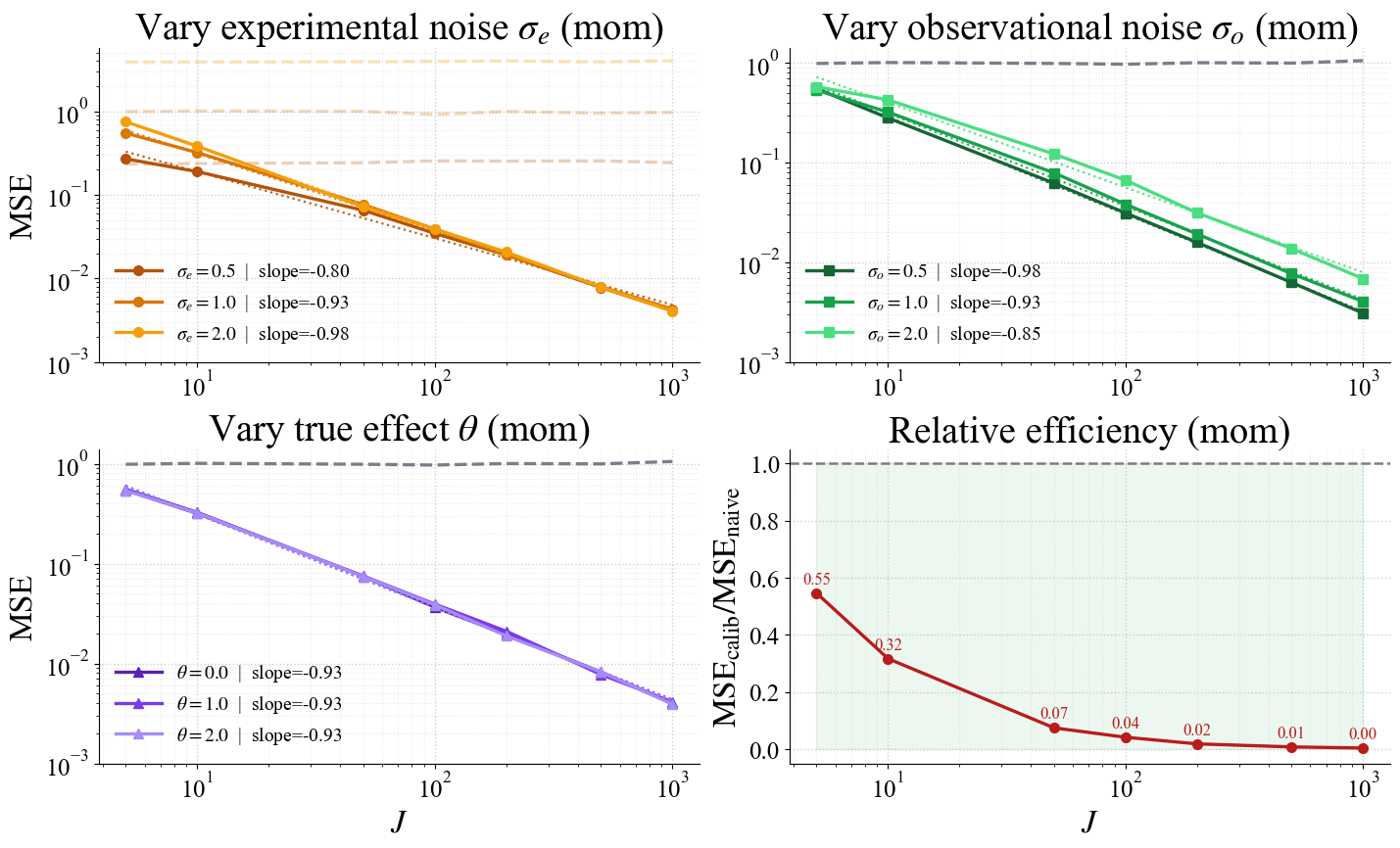
- Simulations (fake data showing the error drops as you add more calibrated studies, roughly like $1/J$ where is the number of observational studies), and
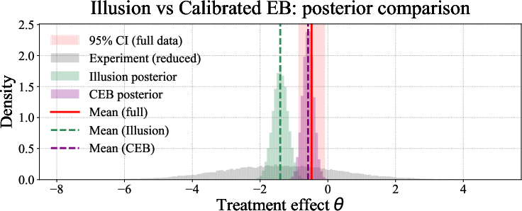
- A semi-real example based on a water-usage experiment in Atlanta. In that example, the “illusion” approach became overconfident around the wrong answer, but the calibrated approach landed near the result from the full, high-quality experiment with reasonable uncertainty.
Why it matters:
- It tells researchers and decision-makers when observational data can truly help and when they can mislead.
- It gives a practical recipe—use calibration/negative controls—to make large, cheap observational datasets actually useful and trustworthy when combined with a smaller, expensive experiment.
So what’s the impact?
This work offers a simple, powerful message with a practical tool:
- Don’t just pile observational studies on top of one experiment and hope for the best.
- Instead, run calibration studies—observational tests where the true effect is known to be $0$—to learn the typical bias of your observational design.
- Use that learned bias to adjust and combine all your studies. Done right, this lets you squeeze real value out of observational data, making your overall answer more accurate and more precise.
In areas like public policy, medicine, education, or tech, where experiments can be limited, this approach can turn “big observational data” from a potential source of confusion into a real engine for better, faster learning.
Knowledge Gaps
Knowledge gaps, limitations, and open questions
Below is a concise list of what remains missing, uncertain, or unexplored, framed to guide actionable future research.
- Real-world feasibility of calibration studies
- How to identify, justify, and implement credible “zero-effect” calibration (negative control) interventions in social, biomedical, and policy settings where true null effects are rare or contestable.
- Practical design guidance for constructing calibration studies that share the same bias-generating mechanisms as target observational studies.
- Validity of the “shared bias distribution” assumption
- Methods to test, diagnose, and quantify departures from the assumption that observational and calibration studies draw study-specific biases from the same population distribution.
- Sensitivity analysis frameworks that characterize estimator degradation when calibration and observational bias distributions differ (e.g., location/scale shifts, skewness, heavy tails).
- Distinguishing bias from true effect heterogeneity
- Extensions that allow study-specific causal effects (random effects) in addition to study-specific biases, and identification strategies to disentangle the two without strong, unverifiable assumptions.
- Designs using multiple calibration conditions or meta-data on study designs to separately identify heterogeneity in effects versus heterogeneity in biases.
- Robustness to model misspecification
- Relax the Gaussian assumptions for both sampling distributions and bias priors (e.g., skewed/heavy-tailed, mixture, or nonparametric priors) and evaluate performance under misspecification.
- Develop robust EB procedures (e.g., Huberized likelihood, α-divergence, or median-based moment-matching) to mitigate undue influence of outlying studies.
- Unknown or misspecified within-study variances
- Theoretical and practical extensions when per-study sampling variances (σe2, σ{o,j}2, σ_{c,k}2) are estimated with error, heterogeneous, or partially missing.
- Joint estimation procedures that propagate variance uncertainty and maintain valid risk/coverage properties.
- Dependence across studies
- Methods that account for correlation among study estimates (shared data sources, overlapping populations, common measurement systems), including cluster- or network-structured dependence in biases.
- Impact of cross-study dependence on EB hyperparameter estimation and posterior contraction.
- Selection and publication biases
- Incorporate selection models for which observational (and calibration) studies are observed or reported, and assess identifiability/robustness of the bias distribution under selective availability.
- Generalized outcome/treatment settings
- Extensions beyond normal means to GLMs, time-to-event outcomes, counts, binary outcomes, and non-linear causal estimands (e.g., risk ratios), including asymptotic and finite-sample guarantees.
- Handling multi-arm treatments, continuous exposures, and interference/spillovers within the EB–calibration framework.
- Transportability and target population alignment
- Methods to reconcile differences in target populations and estimands across experimental, observational, and calibration studies (e.g., weighting/transportability adjustments integrated with EB).
- Conditions under which calibration-derived bias distributions transport across domains, time periods, or measurement systems.
- Design and power calculations for calibration
- Sample size formulas and trade-off analyses for the number and precision of calibration versus observational studies to achieve desired MSE or coverage.
- Adaptive designs that allocate effort between calibration and observational studies based on interim EB hyperparameter uncertainty.
- Diagnostics and goodness-of-fit
- Practical diagnostics (e.g., posterior predictive checks, QQ plots, residual analyses) to assess the adequacy of the fitted bias prior and the match between calibration and observational studies.
- Model comparison tools to choose among candidate bias priors (Gaussian vs mixtures vs nonparametric).
- Finite-sample behavior and coverage
- Systematic study of finite-sample bias, variance, and coverage under small J and K, including the impact of non-negativity constraints in moment estimators (e.g., truncated γ̂2).
- Calibration of credible intervals to achieve nominal frequentist coverage under EB hyperparameter uncertainty.
- Multiple experiments and hierarchical structuring
- Extending the framework to combine multiple randomized experiments with many observational and calibration studies, including hierarchical modeling of experiment-level heterogeneity.
- Borrowing strength across related interventions/designs while allowing design-specific bias distributions.
- Negative control validity and diagnostics
- Tools to verify that negative controls have no direct effect and to quantify small departures from “zero effect” (partial violations), with corrected estimators and uncertainty quantification.
- Design patterns for internal versus external negative controls and their relative strengths/limitations.
- Leveraging study-level covariates
- Modeling bias as a function of observable study characteristics (design choices, adjustment sets, measurement quality), enabling conditional EB priors and targeted shrinkage.
- Variable selection for study-level predictors of bias and causal structure-aware priors that exploit DAG-informed design features.
- Computation and scalability
- Algorithms and software for scalable EB estimation with many studies, high-dimensional study-level covariates, and non-Gaussian priors/likelihoods (e.g., variational EB, stochastic EM).
- Stability and convergence guarantees for marginal likelihood optimization under complex priors.
- Broader sources and types of bias
- Incorporation of measurement error, outcome misclassification, time-varying confounding, model extrapolation bias, and missing data mechanisms into the bias distribution framework.
- Joint modeling of multiple bias mechanisms with identifiable components through a suite of distinct calibration/negative-control designs.
- Empirical validation at scale
- Large-scale applications across domains (medicine, economics, public policy) using real negative controls to assess external validity, robustness, and decision relevance of calibrated EB.
- Benchmarks against alternative data-fusion methods (transportability, bias correction, surrogate outcomes) under matched conditions.
- Guidance for practitioners
- Protocols for selecting calibration interventions, verifying assumptions, diagnosing violations, and reporting uncertainty in applied settings.
- Clear recommendations for when observational data should be down-weighted or excluded based on diagnostics of calibration mismatch.
- Ethical and logistical constraints
- Exploration of ethical, legal, and logistical limits to running calibration studies (especially when “null” interventions may still affect behavior), and alternatives when true negatives are infeasible.
Practical Applications
Immediate Applications
Below are specific, deployable use cases that leverage the paper’s calibrated empirical Bayes (CEB) framework—using calibration/negative-control studies to estimate the bias distribution—and then combine observational and experimental evidence to improve causal estimates.
- Healthcare and pharmacoepidemiology (post-market RWE augmentation)
- Use case: Combine small RCTs with large-scale observational studies (EHRs, claims) to estimate treatment effects on effectiveness and safety. Fit the bias distribution with negative-control outcomes/exposures (assumed null effects) and then shrink observational estimates toward the RCT using CEB.
- Tools/products/workflows: R/Python library implementing (i) moment-matching or marginal-likelihood estimation of bias mean/variance from negative controls, (ii) CEB posterior for target effect; integration with OHDSI/OMOP pipelines; modules for coverage diagnostics and sensitivity analyses.
- Assumptions/dependencies: Availability of valid negative controls that share the same bias mechanism as the observational designs; known or well-estimated standard errors for each study; approximate normality of estimators; stability of bias over time/settings; independence or controlled dependence across studies.
- Online experimentation and product analytics (A/B testing platforms)
- Use case: Combine a gold-standard randomized A/B test with many observational estimates from non-random rollouts or feature toggles. Run “placebo” experiments (e.g., invisible UI flags, holdout metrics expected to be unaffected) as calibration to learn the bias distribution and improve overall effect estimates.
- Tools/products/workflows: Platform module to register and run negative controls alongside standard experiments; CEB estimator embedded in experiment analysis dashboards; sample-size calculators that exploit the O(1/J) MSE gain from adding more observational+calibration studies.
- Assumptions/dependencies: Placebo interventions truly have zero effect on the target metric; logging-based variances are correct; rollouts and calibration studies draw from the same bias process (e.g., same targeting/selection mechanisms).
- Digital advertising and marketing measurement
- Use case: Combine randomized lift tests (e.g., geo or user-level holds) with observational campaign data at scale. Use “ghost ads” or pseudo-exposures (expected nulls) as calibration studies to learn bias from selection into ad exposure, then apply CEB to estimate campaign causal lift more precisely.
- Tools/products/workflows: Measurement SDK that tags negative controls and computes calibrated priors; CEB-based reporting for lift with uncertainty intervals; governance checklist that prevents “illusion of learning” (overconfidence without calibration).
- Assumptions/dependencies: Valid null controls (e.g., ghost ads not delivered); stable selection mechanism; correct variance estimation for aggregated lift estimates.
- Utilities, energy, and water (customer engagement and demand response)
- Use case: As in the paper’s water-usage example, combine a randomized pilot (e.g., conservation nudges) with many observational evaluations across neighborhoods or time. Construct pseudo-treatments (placebos) shaped by the same propensity rules to estimate bias and apply CEB for the target effect.
- Tools/products/workflows: Utility analytics workflow with a “calibration arm” (pseudo-treatments); standard operating procedure (SOP) for bias estimation and CEB combination; dashboards that compare experimental-only vs calibrated estimates.
- Assumptions/dependencies: Pseudo-treatments truly have no effect; observational and calibration studies share the bias-generating process (e.g., same targeting logic).
- Public policy evaluation (social programs and administrative data)
- Use case: Combine small RCTs or pilot experiments with large observational analyses of program rollouts (job training, housing vouchers, tax credits). Use negative-control “pseudo-policies” or placebo timing/place assignments (e.g., fake start dates, fake geographies) as calibration.
- Tools/products/workflows: Policy analytics toolkit that automates creation of placebo policies; CEB estimator in agency dashboards; reporting standards requiring calibration-based bias estimation when combining data sources.
- Assumptions/dependencies: Plausible construction of null/placebo policies; matched administrative data structures; bias stability across geographies/time.
- Education and edtech
- Use case: Combine randomized classroom pilots with large-scale observational data from LMS logs. Use “sham” content versions or metrics expected to be unaffected as negative controls to learn biases due to selection and engagement, then CEB for treatment effects.
- Tools/products/workflows: LMS add-on for calibration experiments; automatic computation of bias priors; guidance for instructors on safe negative-control design.
- Assumptions/dependencies: Negative controls are truly inert; users cannot detect sham content in ways that affect target outcomes.
- Academic meta-research and methods
- Use case: Meta-analytic pipelines that include multiple observational studies plus an anchor RCT, augmented with calibration studies to estimate the observational bias distribution before pooling.
- Tools/products/workflows: Open-source CEB meta-analysis package; preregistration templates that require (i) bias calibration plan, (ii) EB prior estimation approach, (iii) reporting of calibrated vs uncalibrated results.
- Assumptions/dependencies: Observational studies and calibrations are comparable by design; sufficient number of calibrations to stably estimate bias mean/variance.
- Personal health and behavioral apps (N-of-1 measurement)
- Use case: Combine small randomized self-experiments (e.g., timing of caffeine, sleep routines) with ongoing observational tracking. Incorporate sham interventions (e.g., placebo reminders) as negative controls to calibrate bias and refine personal effect estimates through CEB.
- Tools/products/workflows: Consumer-facing app feature to run “placebo days”; automatic bias-prior learning and calibrated effect summaries; user education on negative controls.
- Assumptions/dependencies: Placebo actions do not meaningfully affect outcomes; enough repeated measures to estimate variances; within-person bias stability.
- Risk management and finance (event studies and policy shocks)
- Use case: Combine randomized natural experiments (rare) or lottery allocations with many observational event studies. Use null event windows or non-affected securities/markets as negative controls to learn the bias distribution in selection and model misspecification before CEB pooling.
- Tools/products/workflows: Event-study suite that tags null windows/securities; CEB posteriors for treatment effects with uncertainty reporting; sensitivity checks for volatility/heteroskedasticity.
- Assumptions/dependencies: Selected negative controls have no effect; bias mechanism similar across events/sectors; correct or robust variance estimation.
- Guardrail: avoiding the “illusion of learning”
- Use case: Add an automated check that prevents EB pooling of observational and experimental estimates unless the bias prior is calibrated from negative controls; otherwise, report that observational data do not change the posterior mean and may spuriously reduce variance.
- Tools/products/workflows: “CEB readiness” flag in analysis platforms; compliance rules for evidence synthesis in industry/academia.
- Assumptions/dependencies: Access to candidate negative controls; enforceable governance practices.
Long-Term Applications
The items below require further research, scaling, or development (e.g., generalized models, infrastructure, standards).
- Regulatory evidence standards and guidance (e.g., FDA, EMA, NICE)
- Vision: Formalize CEB with negative controls as an accepted pathway to combine RCTs and RWE, including checklists for calibration quality, sensitivity analyses, and bias-stability diagnostics.
- Dependencies: Consensus on negative-control validation; standard APIs for data provenance and variance estimation; sector-wide benchmarking studies.
- Cross-institution bias registries (“BiasBank”)
- Vision: Shared repositories of bias distributions for common observational designs (propensity rules, data sources) within sectors (healthcare, education), enabling reuse of priors and faster calibration for new studies.
- Dependencies: Data-sharing agreements, privacy/federated learning setups, common ontologies for study design metadata.
- Federated and privacy-preserving CEB
- Vision: Learn shared bias distributions across hospitals/platforms without pooling raw data; apply CEB locally for each site’s target effect.
- Dependencies: Federated marginal-likelihood/moment-matching algorithms; robust aggregation against site heterogeneity.
- Robust and generalized models
- Vision: Extend beyond Gaussian normal-means models to GLMs, survival, longitudinal and network settings; incorporate heavy-tailed or mixture priors for biases; allow study clustering with design-level random effects.
- Dependencies: Theory for risk guarantees under non-normal outcomes; scalable Bayesian inference; diagnostics for model misspecification.
- Heterogeneity-aware CEB (subgroup- or context-specific biases)
- Vision: Estimate bias priors by subgroup (e.g., geography, demographics) or by study design family, enabling calibrated pooling that respects heterogeneity.
- Dependencies: Larger libraries of calibration studies per subgroup; partial pooling hierarchies; model selection criteria for grouping.
- Adaptive calibration design
- Vision: Actively select the most informative negative controls to reduce posterior uncertainty fastest (optimal design for calibration studies).
- Dependencies: Sequential design algorithms, cost/benefit models, platform support for quick turnaround experiments.
- Real-time/streaming CEB
- Vision: Continuously update bias priors and calibrated estimates as new observational and calibration studies arrive (e.g., online services and marketplaces).
- Dependencies: Streaming inference infrastructure; drift detection for bias-process changes; alerting systems when recalibration is required.
- Integration with modern causal ML
- Vision: Pair CEB with doubly robust/meta-learner estimators to account for high-dimensional confounding; use negative controls to calibrate residual biases from model selection/regularization.
- Dependencies: Interfaces between causal ML pipelines and CEB modules; robustness to variance under cross-fitting.
- Automated discovery of negative controls
- Vision: Algorithmic or LLM-assisted discovery and validation of candidate null exposures/outcomes (e.g., text-mined clinical concepts likely to be unaffected).
- Dependencies: High-quality ontologies; validation datasets; safeguards against spurious “nulls”.
- Governance and education
- Vision: Industry and academic SOPs that mandate calibration studies when combining experimental and observational evidence; training modules that demonstrate the “illusion of learning” and the CEB remedy.
- Dependencies: Adoption by journals, IRBs, data officers; case libraries for teaching; reproducibility toolkits.
- Robotics and offline reinforcement learning (exploratory)
- Vision: Combine limited randomized interventions (safe exploration) with large logged observational data from policies; define null actions or metrics expected to be unaffected as negative controls to learn bias from confounding in off-policy evaluation, then apply CEB.
- Dependencies: Domain-specific nulls that do not influence dynamics; sequential dependence accounted for in theory; variance estimation for off-policy estimators.
- Personalized decision support
- Vision: Calibrated N-of-1 tools for clinicians/consumers that seamlessly mix randomized micro-trials with passive data and embedded negative controls; deliver individualized causal estimates with transparent uncertainty.
- Dependencies: Sufficient repeated measures; behaviorally sound placebo/sham designs; on-device or private CEB inference.
In all cases, the central dependency is the availability and validity of calibration/negative-control studies that share the same bias-generating mechanisms as the observational studies feeding the causal estimate. Without this alignment, the “illusion of learning” can persist or be exacerbated.
Glossary
- Asymptotically normal: A property where an estimator’s sampling distribution approaches a normal distribution as sample size increases. Example: "the sampling distribution of causal estimators is often asymptotically normal;"
- Average Treatment Effect (ATE): The expected difference in outcomes between treatment and control conditions in a population. Example: "Our target estimand is the average treatment effect (ATE) of the T3 message on 2008 summer water usage,"
- Bias adjustment: Techniques for correcting systematic errors in estimates due to confounding or other biases. Example: "Existing approaches use transportability assumptions, bias adjustment, shrinkage, reweighting, or surrogate outcomes"
- Calibrated empirical Bayes (CEB): An empirical Bayes approach that uses calibration studies (negative controls) to estimate the bias distribution before combining observational and experimental data. Example: "The result is a calibrated empirical Bayes procedure for causal estimation from experimental and observational studies."
- Calibration studies: Observational analyses of interventions with known null effects used to learn the distribution of biases. Example: "Calibration studies help solve our problem because they provide direct information about the distribution of biases associated with a given observational design."
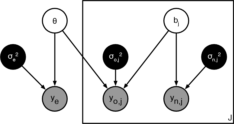
- Causal graphs: Graphical models (often DAGs) representing causal relationships among variables. Example: "summarizes the experimental, observational and calibration designs using causal graphs."
- Causal inference: Methods for drawing conclusions about causal relationships from data. Example: "When randomized experiments are infeasible, scientists often resort to observational studies for causal inference."
- Consistency: An estimator’s property of converging to the true value as sample size grows. Example: "(See Theorem ... in the Appendix for results about the risk and consistency of the EB procedure.)"
- Credible interval: A Bayesian interval estimate for a parameter reflecting posterior uncertainty. Example: "a tighter 95% credible interval of [-0.90,-0.27]"
- Empirical Bayes: A framework that estimates prior distributions from repeated data to improve inference. Example: "Empirical Bayes is a natural framework for this problem"
- Estimand: The target quantity a procedure aims to estimate. Example: "We define the calibration estimand as the difference in outcomes between the pseudo‑treated and pseudo‑control groups,"
- Hierarchical Bayesian models: Bayesian models with parameters organized in multiple levels, allowing pooling/sharing across groups. Example: "Graphical representations of the hierarchical Bayesian models."
- Hierarchical Gaussian model: A hierarchical model where conditional distributions are Gaussian. Example: "we formalize the illusion of learning from observational data in a hierarchical Gaussian model for one experimental estimate and many observational estimates."
- Ignorability assumption: The assumption that, conditional on observed covariates, treatment assignment is independent of potential outcomes. Example: "Because treatment assignment was randomized at the household level, the ignorability assumption ... holds."
- Improper prior: A prior distribution that does not integrate to one (e.g., flat prior), used for noninformative Bayesian analysis. Example: "note the flat (improper) prior on θ"
- Informative prior: A prior distribution that encodes substantive information about parameters. Example: "if we held an informative prior—then observational studies could contribute to the estimate of the causal effect."
- Marginal likelihood: The likelihood of observed data integrated over latent parameters, used for hyperparameter estimation. Example: "maximizing the marginal likelihood"
- Method of moments: An estimation method matching sample moments to theoretical moments to estimate parameters. Example: "While our calibrated EB estimates are based on the method of moments"
- Moment matching: Choosing parameters so model-implied moments equal empirical moments. Example: "In our theory and simulations ..., we also use moment matching."
- Negative controls: Variables or interventions known to have no causal effect, used to detect and quantify bias. Example: "our calibration studies are close in spirit to negative controls and related diagnostic tools"
- Normal means model: A model where observations are normally distributed around unknown means with known variances. Example: "The normal means model is a reasonable theoretical device:"
- Oracle: A benchmark method that uses the true (unknown) parameters as if they were known. Example: "Oracle: Uses the true hyperparameters (μ⋆, γ2⋆)."
- Overlap assumption: The condition that each unit has a nonzero probability of receiving each treatment level. Example: "The overlap assumption ... is also satisfied since all households have positive probability to receive the treatment or control."
- Posterior: The probability distribution of parameters after observing data. Example: "The posterior p(θ y_{e}, y_{o}) is a normal distribution,"
- Posterior mean: The expected value of a parameter under the posterior distribution, often used as a point estimate. Example: "The posterior mean is"
- Posterior variance: The variance of a parameter under the posterior distribution, quantifying uncertainty after observing data. Example: "The posterior variance is"
- Potential outcomes: The outcomes that would be observed under each possible treatment assignment for a unit. Example: "We write O_i(a) for the potential outcome"
- Propensity score model: A model for the probability of treatment given covariates, used to adjust for confounding. Example: "a new propensity score model e_{o}(X) := ℙ_{o}(A = 1 ∣ X)"
- Relative efficiency: The ratio of mean squared errors (or variances) of two estimators, measuring comparative precision. Example: "Relative efficiency (RE), defined as the ratio between the MSE of the calibrated empirical Bayes estimator and that of the experimental estimator"
- Reweighting: Adjusting sample weights to emulate a target distribution or assignment mechanism. Example: "We reweight the samples in B_j so that the empirical distribution of {X_i, A_i} matches {X_i, e_o(X_i)}."
- Risk: Expected loss of an estimator; here, expected squared error relative to the true parameter. Example: "The risk is equal to the variance of the experiment"
- Sample splitting: Dividing data into parts to estimate different components or to avoid overfitting in inference. Example: "it uses sample splitting to show the results."
- Semi-synthetic: Combining real data with simulated components to create a controlled empirical study. Example: "a semi-synthetic application based on ferraro2013heterogeneous's water-usage experiment."
- Shrinkage: Pulling noisy estimates toward a central value (e.g., via priors) to reduce variance. Example: "allows observational studies to inform the estimation of causal parameters via empirical Bayes shrinkage."
- Surrogate outcomes: Auxiliary outcomes used to link or transfer information across studies or settings. Example: "use transportability assumptions, bias adjustment, shrinkage, reweighting, or surrogate outcomes"
- Transportability assumptions: Assumptions enabling causal effects learned in one setting to be validly applied in another. Example: "Existing approaches use transportability assumptions, bias adjustment, shrinkage, reweighting, or surrogate outcomes"
- Vanishing risk: Risk that approaches zero as the amount of data (e.g., number of studies) increases. Example: "achieves asymptotically vanishing risk as we see more observational and calibration studies,"
Collections
Sign up for free to add this paper to one or more collections.

