Systematic and Statistical Uncertainties in the Non-Gravitational Acceleration of 3I/ATLAS
Abstract: We present a detailed analysis of the trajectory of the interstellar comet 3I/ATLAS, focusing on its non-gravitational acceleration (NGA) parameters and their uncertainties. Orbital solutions are computed with models that implement symmetric, time-offset, and asymmetric radial dependence of the outgassing law relative to perihelion. We assess solution robustness through multiple data-selection strategies and comparison with independent determinations. The radial and normal NGA components (A_1 and A_3) are broadly consistent across all configurations, whereas the transverse component (A_2) is more sensitive to data selection, parameter correlations, and orbital phase coverage. Models with asymmetric radial decay slopes marginally improve the fit, but they also introduce additional degeneracies, contributing to systematic uncertainties. The magnitude of the NGA scaled to 1 au constrains the nucleus size of 3I. While our total acceleration estimates agree well with that of JPL's Small-Body Database solution, inclusion of systematic modeling effects implies a significantly larger uncertainty in the inferred radius of 3I.


Paper Prompts
Sign up for free to create and run prompts on this paper using GPT-5.
Top Community Prompts
Explain it Like I'm 14
A simple explanation of “Systematic and Statistical Uncertainties in the Non‑Gravitational Acceleration of 3I/ATLAS”
What this paper is about (big picture)
This paper studies the path of an interstellar comet called 3I/ATLAS (the third interstellar object found passing through our Solar System). The main focus is on tiny “extra” pushes on the comet that don’t come from gravity—caused by gas and dust blasting off its surface when it warms up near the Sun. These gentle pushes are called non‑gravitational accelerations (NGAs). By measuring them carefully, the authors try to understand how 3I moves, how big its solid core (nucleus) might be, and what that tells us about comets from other star systems.
What questions the researchers asked
The authors set out to answer a few clear questions:
- How strong are the tiny rocket‑like pushes (NGAs) on 3I, and in what directions do they act?
- Do these pushes change before and after the comet’s closest approach to the Sun (perihelion), and do they peak exactly at perihelion or a bit early/late?
- How much do the answers depend on which observations are used and on the details of the mathematical model?
- What do these pushes tell us about the comet’s size?
How they did the study (in everyday language)
The team used thousands of observations of 3I’s position in the sky from May 2025 to February 2026, taken by telescopes on Earth and in space (including TESS and Hubble) and even from deep‑space spacecraft (Psyche and the Trace Gas Orbiter). Then they tried different “recipes” (models) to describe how 3I moves:
- Gravity‑only model: assumes only the Sun and planets pull on the comet.
- NGA models: add tiny extra pushes from outgassing (like miniature jets):
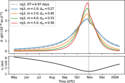
- Symmetric model: the push gets strongest at perihelion and decreases the same way before and after.
- Offset‑peak model: the push reaches its maximum a few days before or after perihelion.
- Asymmetric‑slope model: the push fades with distance differently before versus after perihelion (not the same slope on both sides).
To picture the directions of the pushes, imagine three arrows tied to the comet:
- A1 points toward/away from the Sun (radial).
- A2 points along the comet’s path, like a gentle tailwind or headwind (transverse).
- A3 points “up or down” out of the comet’s orbital plane (normal).
They used:
- Least‑squares fitting: like drawing the best‑fit line through data points, but in many dimensions, to find the best values of A1, A2, A3.
- MCMC (Markov Chain Monte Carlo): a way to explore many possible solutions to see how uncertain each parameter is.
- Jackknife tests: re‑fitting after removing certain chunks of data (like specific time ranges or particular observatories) to check if any one piece of data overly influences the result.
They also checked for measurement quirks (like a small timing offset from one station) and tested whether changing the model details changed the answers.
What they found and why it matters
Here are the main results:
- Gravity alone doesn’t explain the data. Adding NGA (the outgassing push) clearly improves the fit to the comet’s path. In other words, 3I is being nudged by its own jets.
- The size of the total push near Earth’s distance from the Sun (1 au) is tiny but measurable, around a few times 10⁻⁸ au/day². That’s extremely small—think of a whisper of a shove—but over weeks and months it adds up enough to notice.
- The push toward/away from the Sun (A1) and the “up/down” push (A3) are fairly consistent across different tests. The along‑path push (A2) is the trickiest: it changes more depending on which data you include and which model you use. That makes A2 the most uncertain.
- Allowing the push to be a bit asymmetric around perihelion or to peak slightly before/after perihelion gives only a small improvement to the fit, but it introduces “degeneracies.” That means two different explanations (a slope asymmetry vs. a time shift) can look almost the same in the data, so it’s hard to tell which is truly happening.
- A few spacecraft observations (from Psyche and TGO), even though there aren’t many of them, help a lot. Because they observed from different places in the Solar System, they provide a unique angle that tightens the results.
- Their total push estimate is broadly consistent with a trusted external source (JPL’s Small‑Body Database). But when the authors include the extra modeling uncertainties, the error bars on the comet’s size get bigger. Bottom line: 3I’s nucleus is likely around kilometer‑scale, but the exact size is less certain than some earlier estimates suggested.
Why this matters:
- The strength of the push helps estimate the comet’s mass and size (a smaller, lighter comet gets pushed more by the same jets).
- Getting the motion right is crucial to trace where the comet came from and where it’s going—and maybe even link it to a birthplace among the stars.
- Understanding how outgassing behaves (symmetric vs. asymmetric, early vs. late peak) teaches us about the comet’s surface materials, which ices are evaporating, and how sunlight warms and releases them.
What this means going forward
The big takeaways:
- 3I is definitely being nudged by its own outgassing, and we can measure it.
- Some details—especially the sideways (A2) push and whether the outgassing is asymmetric or just time‑shifted—are hard to pin down with the current data. Different modeling choices can lead to different answers that look equally good.
- Because of these modeling uncertainties, size estimates should include bigger error bars. More observations, especially from different vantage points and across a wider range of distances from the Sun, would help break the ties between competing explanations.
- As we discover more interstellar visitors, these methods will help us quickly and reliably figure out their paths, their physical properties, and clues to their origins in other solar systems.
Knowledge Gaps
Knowledge gaps, limitations, and open questions
The paper identifies several sources of statistical and systematic uncertainty but leaves a number of issues unresolved. The following concrete gaps highlight where additional data, analyses, or modeling could materially reduce ambiguity in the non-gravitational acceleration (NGA) of 3I/ATLAS and its physical interpretation:
- Insufficient constraint on the radial dependence of activity, : the strong degeneracy among the average slope , the asymmetry parameter , and the total NGA magnitude persists because the current arc samples a limited range of heliocentric distances; additional astrometry at larger post-perihelion distances (beyond ≈4 au) and late-time observations are needed to break this degeneracy.
- Unresolved degeneracy between a shifted NGA peak () and asymmetric pre-/post-perihelion slopes (): both parameterizations fit the data similarly and project onto the same observable; joint analyses with contemporaneous activity tracers (e.g., gas production curves, thermophysical models) are required to distinguish true peak offsets from slope asymmetry.
- Sensitivity and inconsistency of the transverse component : varies significantly with data selection and differs between pre- and post-perihelion fits; targeted, denser astrometry near perihelion and improved phase coverage are needed to stabilize and diagnose whether the variation is physical or methodological.
- Over-reliance on a small number of deep-space astrometric points (Psyche/TGO): NGA estimates (especially ) shift noticeably when these are removed; independent spacecraft or heliocentric platforms and reprocessing of these measurements are needed to validate their influence and reduce single-dataset leverage.
- Station timing biases not globally modeled: a ≈43 s timing offset at station M47 was identified ad hoc, but no systematic, per-station timing-offset estimation was performed; incorporate station-specific clock-offset parameters or re-reduce time stamps to mitigate hidden systematics.
- Simplified NGA formalism: the Marsden-style, constant-parameter RTN model assumes fixed , , and smooth ; it does not capture rotational modulation, evolving jet geometries, or seasonal effects; develop and test time-variable (e.g., periodic) NGA models tied to the observed ≈7.1 h rotation and jet morphology.
- Absence of non-gravitational torque modeling: the study does not attempt to constrain spin-state changes from astrometry; couple force and torque models (informed by jet imaging and spin axis orientation) to assess whether torques are detectable and how they correlate with .
- Lack of physically based sublimation/thermophysical models: aside from and a phenomenological slope asymmetry, no composition- or insolation-driven models are fit; fit thermophysical models (CO/CO₂/H₂O mixtures with thermal lag and seasonal illumination) jointly to astrometry and production rates to reduce model-form uncertainty.
- No joint fit to activity measurements: astrometric NGA inferences are not combined with gas/dust production data, which remain controversial; a hierarchical joint inversion (astrometry + spectroscopy/photometry) could directly constrain , , and .
- Unreconciled discrepancy in with JPL SBDB solution: the paper notes large differences in but does not perform a controlled, harmonized re-fit using a matched dataset and identical weighting/de-biasing to isolate the source of disagreement.
- Error model limitations: weights assume uncorrelated, Gaussian errors (diagonal ); potential intra-night correlations, catalog systematics, and heavy tails are not modeled; adopt hierarchical Bayesian weighting, per-station error floors, and robust likelihoods to quantify their impact on .
- Outlier treatment sensitivity not fully quantified: the Carpino et al. rejection is used, but alternative robust estimators (e.g., Huber/Tukey, mixture models) are not compared; perform method-of-estimators cross-checks to assess stability of and .
- Restricted post-perihelion coverage (to ≈4.05 au): the asymmetric-slope fits favor –4 but remain weakly discriminating; late-time recovery (e.g., 5–7 au post-perihelion) would test steepness and asymmetry directly.
- Propagation of model-choice uncertainty into nucleus size is incomplete: while the paper notes that systematic modeling broadens size uncertainty, it does not deliver a posterior on radius that marginalizes over , , , and error models; provide a fully marginalized size estimate under explicit physical assumptions (density, active fraction, momentum transfer).
- Impact of NGA modeling on the reconstructed incoming asymptote is not quantified: the paper states its importance but does not map how different NGA parameterizations shift the direction; compute the distribution of asymptotic state vectors under competing models to bound provenance inferences.
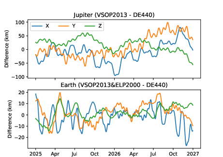
- Limited validation of the dynamical environment: planetary positions are from analytical theories (VSOP2013/ELP2000) rather than modern numerical ephemerides (e.g., DE440); although Appendix tests suggest adequacy, a quantified comparison of induced changes in versus formal errors would solidify this assumption.
- Radiation pressure and solar-wind forces on dust coma not explicitly bounded: while likely subdominant for a kilometer-scale, active nucleus, the paper does not provide upper limits; place quantitative bounds to ensure these do not alias into /.
- Catalog de-biasing dependence untested: only one de-biasing scheme is used; re-fit with alternative catalog de-biasing (e.g., Gaia-based corrections) to assess sensitivity of and .
- No systematic solution for station-dependent astrometric systematics beyond timing: per-station position biases, plate-scale errors, or chromatic refraction are not modeled; include station-level nuisance parameters or re-reduce key datasets.
- Potential fragmentation or outburst episodes not incorporated: the NGA model assumes smooth behavior; examine residuals for transient signatures and, if present, include episodic activity terms.
- Lack of a jet-resolved force model: high-resolution imaging suggests localized jets; a forward model that maps specific jet locations and spin geometry to RTN force components could directly test whether is physically plausible.
- Covariance between initial state and NGA parameters not propagated to predictive ephemerides: provide epoch-dependent sky-plane uncertainty growth under different NGA models to guide future observing strategies.
- Priors are minimal and not physics-informed: uniform bounds on allow broad, weakly constrained regions; introduce physics-based priors (e.g., momentum-coupling efficiencies, plausible active fractions) to regularize ill-conditioned fits.
- Discrepancies in water production rates across studies remain unresolved: the paper cites controversy but does not adjudicate; coordinated, cross-calibrated spectroscopy/UV observations are needed to anchor and validate /.
These gaps suggest clear follow-ups: extend the astrometric arc (especially post-perihelion), obtain additional heliocentric-vantage astrometry, jointly model astrometry with activity and thermophysics, introduce more realistic and time-variable force models, and harmonize data processing across teams to reconcile parameter discrepancies—particularly for and the interpretation of NGA asymmetry.
Practical Applications
Immediate Applications
The paper’s methods and findings can be operationalized now across observation, orbit-determination, and decision-support workflows:
- Upgrade orbit-determination pipelines to be “NGA-aware”
- Use cases: Incorporate symmetric (ng1), time-offset (ng2), and asymmetric-slope (ng3) non‑gravitational acceleration models in standard orbit solutions; propagate both statistical and systematic uncertainties to ephemerides.
- Sectors: Aerospace/defense (SSA/planetary defense), academia (celestial mechanics), software (astrodynamics libraries).
- Tools/products/workflows: Integrate heyoka’s Taylor Adaptive integrator and automatic differentiation; extend orbit_finder with MCMC and jackknife modules; add ensemble model runs (ng1/ng2/ng3) to ephemeris products.
- Assumptions/dependencies: Access to ADES-formatted observations; computational resources for sampling; community acceptance of multiple-model ephemerides; the 1/r² baseline is appropriate unless otherwise indicated by data.
- Robust uncertainty quantification for small-body trajectories
- Use cases: Combine covariance-based errors with MCMC posterior sampling and jackknife stress tests to capture parameter correlations and model degeneracies (e.g., between , , and ).
- Sectors: Aerospace/defense (impact probability, mission design), academia (statistical astrodynamics).
- Tools/products/workflows: UQ dashboards showing posterior cones and sensitivity to data subsets; automated reporting of systematic bands alongside statistical errors.
- Assumptions/dependencies: Sufficient phase coverage; quality-controlled astrometry; reproducible pipelines.
- Observation planning that targets sensitivity windows
- Use cases: Prioritize pre- and post-perihelion coverage and heliocentric distance diversity to constrain and asymmetries; schedule follow-up around conjunction gaps.
- Sectors: Observatory operations, survey programs.
- Tools/products/workflows: Scheduling heuristics that maximize information gain on and ; notification to re-allocate time when gaps threaten degeneracy.
- Assumptions/dependencies: Flexible scheduling; access to multiple facilities; timely data reduction.
- Leverage deep-space vantage points to reduce NGA uncertainty
- Use cases: Opportunistic target-of-opportunity (ToO) imaging from interplanetary spacecraft (e.g., Psyche, TGO) to break geometry degeneracies and tighten .
- Sectors: Mission operations, planetary defense coordination (NASA/ESA).
- Tools/products/workflows: Standing ToO protocols; fast pointing requests; small-body tracking “beacon” roles for cruise-phase spacecraft.
- Assumptions/dependencies: Spacecraft availability, downlink capacity, and attitude constraints; inter-agency coordination.
- Quality control of astrometry via automated timing-offset detection
- Use cases: Detect station-level timing biases (e.g., RA residual clusters explainable by Δt) during ingestion to prevent fit contamination.
- Sectors: Observatory software, data centers (MPC, JPL SBDB).
- Tools/products/workflows: Residual-rate ratio checks; station health flags in ADES pipelines; automated feedback to submitters.
- Assumptions/dependencies: Reliable metadata on exposure timing; initial orbit good enough to compute apparent rates.
- More cautious physical inferences from NGA (e.g., nucleus size)
- Use cases: Report size estimates with enlarged uncertainty bands reflecting model systematics and degeneracies; avoid overconfident claims that drive public policy or media narratives.
- Sectors: Academia, science communication, mission pre‑feasibility.
- Tools/products/workflows: Size-posteriors conditioned on volatile assumptions (CO/CO₂ vs H₂O) and slope asymmetry; comparison reports across models.
- Assumptions/dependencies: Thermal/volatile models used remain the dominant interpretation; photometric constraints available.
- Planetary-defense risk products that include NGA-induced dispersion
- Use cases: For active comets and outgassing NEOs, include NGA uncertainty envelopes in close-approach and impact-probability computations.
- Sectors: Civil protection, governmental agencies.
- Tools/products/workflows: “NGA-on/NGA-off” scenario bracketing; ensemble propagation with model-weighting.
- Assumptions/dependencies: Sufficient observational cadence to constrain NGA before decision windows.
- Performance and reliability improvements in astrodynamics software
- Use cases: Adopt automatic differentiation and Taylor integrators to reduce implementation error and improve runtime for repeated sensitivity evaluations.
- Sectors: Software/compute, commercial astrodynamics.
- Tools/products/workflows: heyoka-backed propagators; CI tests validating integrator precision against DE ephemerides.
- Assumptions/dependencies: Developer expertise; licensing and maintenance of dependencies.
- Standardized weighting and de-biasing in astrometry
- Use cases: Apply Veres et al. (2017) weighting and Eggl et al. (2020) de-biasing broadly to improve fit stability across heterogeneous stations.
- Sectors: Data centers, observatories, academia.
- Tools/products/workflows: Shared configuration files for weights/biases; station-specific profiles.
- Assumptions/dependencies: Up-to-date station performance characterizations; willingness to adopt conservative errors.
Long-Term Applications
These applications require further research, broader infrastructure, or technology development to realize at scale:
- Heliocentric small-telescope network for geometric diversity
- Use cases: Constellations of rideshare CubeSats in inner solar orbit providing continuous, multi-chord astrometry to break NGA degeneracies.
- Sectors: Space industry, policy (international collaboration).
- Tools/products/workflows: Low-cost optical payloads; onboard timing calibration; autonomous data return.
- Assumptions/dependencies: Funding, rideshare opportunities, long-term operations; cross-agency data sharing.
- Rapid-response intercept missions to interstellar objects (ISOs)
- Use cases: NGA-aware mission design and navigation; earlier detection and decision timelines informed by sensitivity of and asymmetry.
- Sectors: Aerospace, planetary science.
- Tools/products/workflows: Trajectory design that robustly handles NGA model ensembles; onboard optical nav to estimate NGA in-flight.
- Assumptions/dependencies: Wide-field survey lead time; rapid-launch capability; technology readiness for fast flybys.
- Physics-based outgassing models integrated into orbit fits
- Use cases: Coupling thermal, shape, spin-state, and volatile sublimation models to reduce reliance on phenomenological and mitigate degeneracies (e.g., vs ).
- Sectors: Academia, software (multiphysics simulation).
- Tools/products/workflows: Data assimilation frameworks that fuse photometry, spectroscopy, and astrometry; GPU-accelerated thermophysical solvers.
- Assumptions/dependencies: High-quality light curves, jet morphology, rotational period data; validation datasets.
- Autonomous NGA estimation and compensation for proximity operations
- Use cases: Spacecraft around active comets/volatile-rich asteroids estimating and compensating for cometary accelerations in real time for navigation and sampling.
- Sectors: Robotics, aerospace.
- Tools/products/workflows: Onboard filters combining optical/range data with NGA process models; safety envelopes that adapt to activity changes.
- Assumptions/dependencies: High-fidelity sensors; flight-proven autonomy stacks; robust power/thermal budgets.
- Community standards for systematic-uncertainty reporting
- Use cases: Ephemeris providers publish ensemble-based uncertainty (statistical + systematic) for small bodies; policy guidance for risk communication.
- Sectors: Policy, data centers, planetary defense coordination bodies.
- Tools/products/workflows: Interoperable metadata for model families; best-practice documents; certification of “decision-grade” products.
- Assumptions/dependencies: Consensus-building across agencies; updates to data formats (e.g., ADES extensions).
- Active-learning schedulers for telescopes
- Use cases: ML-driven tools that choose observation times and stations to maximally reduce uncertainty in the most sensitive parameters (e.g., ).
- Sectors: Software/AI, observatory operations.
- Tools/products/workflows: Bayesian experimental design modules; reinforcement-learning schedulers integrated with observatory queues.
- Assumptions/dependencies: Historical performance data; API access to scheduling systems; validation on live targets.
- Cross-domain transfer of UQ and bias-detection methods
- Use cases: Apply MCMC + jackknife stress-testing and timing-offset diagnostics to GNSS receiver calibration, LEO object tracking, and Earth-observation sensor networks.
- Sectors: Telecom, defense, remote sensing.
- Tools/products/workflows: Generic residual-analysis packages; sensor-fusion toolkits highlighting station/systematic biases.
- Assumptions/dependencies: Access to high-rate residuals and metadata; stakeholder training in statistical diagnostics.
- Commercial analytics for small-body trajectory risk
- Use cases: Insurance and mission-planning services that price risk considering NGA-induced dispersion and data-vantage scenarios.
- Sectors: Finance/insurance, space operators.
- Tools/products/workflows: Scenario simulators with model-weighted forecasts; client dashboards for decision support.
- Assumptions/dependencies: Market demand; reliable data pipelines; clear liability boundaries.
- Open, modular orbit-determination platforms
- Use cases: Community-driven, containerized stacks that combine fast integrators (heyoka), standardized data ingestion, and UQ modules for reproducible results.
- Sectors: Software, academia, industry.
- Tools/products/workflows: Versioned containers; automated provenance and replay; plugin interfaces for new NGA models.
- Assumptions/dependencies: Sustained maintainership; funding for infrastructure; broad adopter base.
Glossary
- ADES (Astrometry Data Exchange Standard): A standardized format for exchanging astrometric measurements and metadata. "reported in the Astrometry Data Exchange Standard (ADES) format."
- affine-invariant ensemble sampler: A Markov-chain Monte Carlo algorithm whose performance is invariant under affine transformations of parameter space. "using the affine-invariant ensemble sampler emcee"
- asymptotic trajectory: The path an object approaches at large distances (e.g., incoming or outgoing hyperbolic branch), used to infer its origin. "to confidently reconstruct the object’s incoming asymptotic trajectory"
- batch least-squares: A parameter estimation method that minimizes the sum of squared residuals over a set (batch) of observations. "using a standard batch least-squares orbit determination procedure"
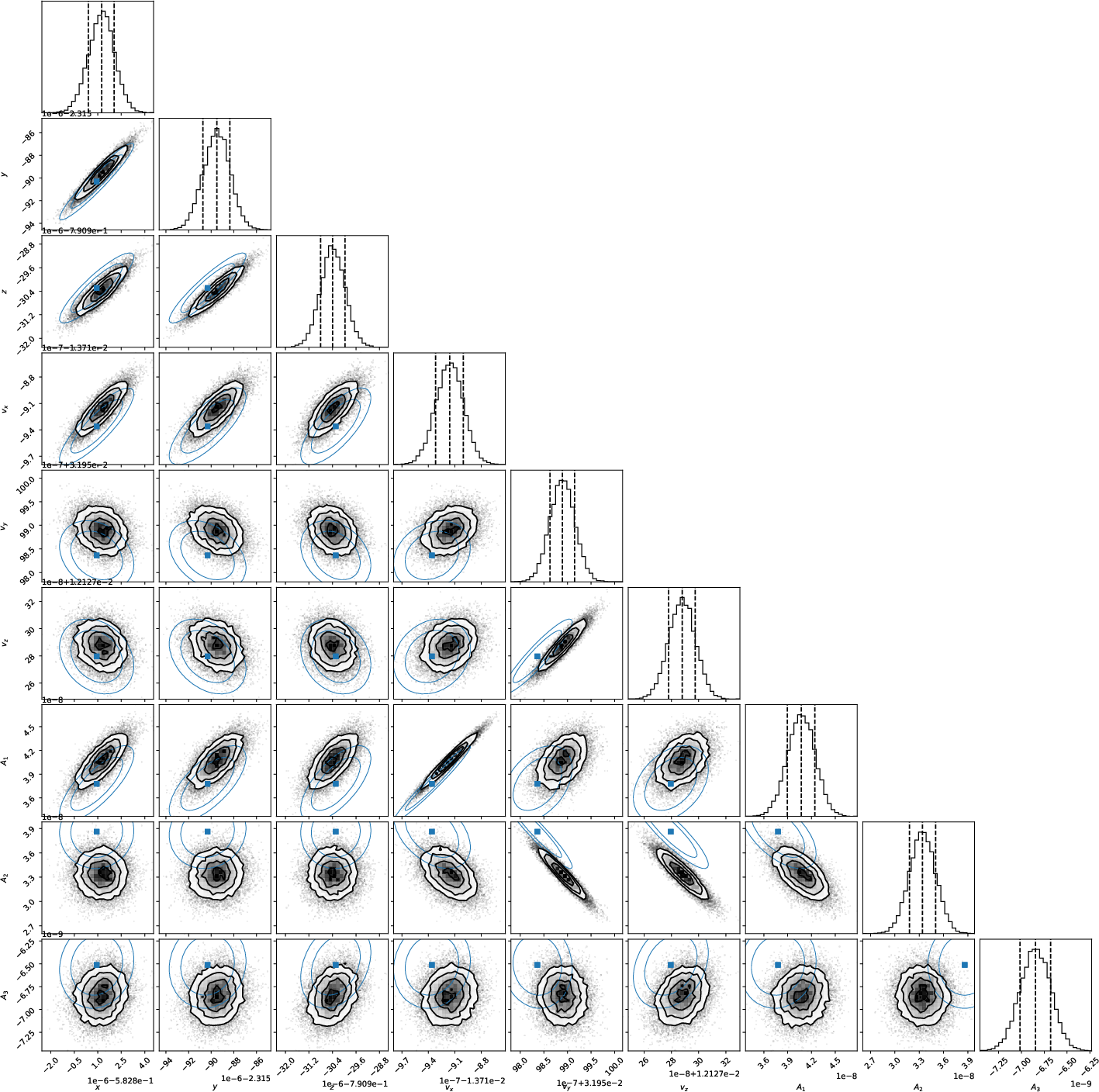
- Cartesian heliocentric state vector: The 6D vector of position and velocity components in Cartesian coordinates with respect to the Sun. "the Cartesian heliocentric state vector (x, y, z, v_x, v_y, v_z)"
- covariance matrix: A matrix encoding uncertainties and correlations among estimated parameters. "where the covariance matrix of the estimated parameters is given by Γ = C{-1}"
- de-biasing: Correcting systematic offsets in observational data to reduce bias. "bias corrections following the de-biasing scheme of \citet{Eggl_ea:2020} were applied where applicable."
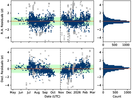
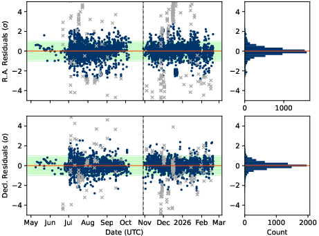
- declination: The celestial coordinate measuring angular distance north or south of the celestial equator. "in right ascension (top panels) and declination (bottom panels)."
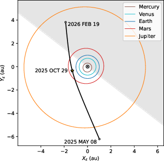
- ecliptic reference frame: A coordinate frame aligned with the plane of Earth’s orbit around the Sun. "Orbit of 3I in the heliocentric ecliptic reference frame."
- ELP2000: An analytical lunar theory used to compute the Moon’s position. "The heliocentric positions of the gravitational perturbers are obtained from the analytical theories VSOP2013 and ELP2000 for the planets (including Pluto) and the Moon, respectively"
- ephemerides: Tables or computed data giving positions of celestial bodies over time. "numerical ephemerides based on more comprehensive dynamical models, such as JPL's DE440"
- equatorial reference frame (J2000): A frame based on Earth’s equator and equinox at the standard epoch J2000. "within a heliocentric equatorial reference frame referred to the J2000 equator and equinox."
- gravitational parameter (μ): The product G·M for a body, governing gravitational acceleration. "where μ_\odot is the gravitational parameter of the Sun."
- hyperbolic trajectory: An unbound orbit with eccentricity greater than 1, indicating interstellar origin if around the Sun. "on a strongly hyperbolic trajectory"
- Jackknife: A resampling technique that assesses sensitivity by systematically removing subsets of data. "we also performed a jackknife analysis using two complementary strategies."
- JPL’s Small-Body Database (SBDB): NASA’s database providing orbital and physical parameters for small Solar System bodies. "JPL’s Small-Body Database (SBDB)"
- Marsden formalism: A standard model for cometary non-gravitational accelerations driven by outgassing. "The non-gravitational component of the acceleration is modeled following the \citet{Marsden_ea:1973} formalism:"
- Markov-Chain Monte Carlo (MCMC): A probabilistic sampling method used to characterize posterior distributions of model parameters. "Markov-Chain Monte Carlo (MCMC) sampling of the posterior probability distribution."
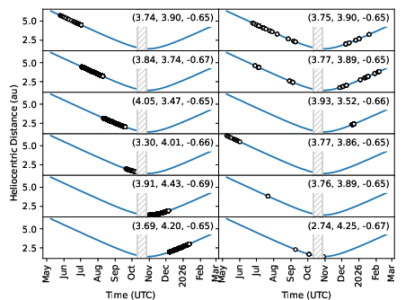
- mean anomaly: An orbital angle parameter proportional to time since periapsis in Keplerian motion. "sliding window of approximately equal size in terms of mean anomaly"
- Minor Planet Center (MPC): The IAU’s center for minor planet observations, orbit determinations, and data dissemination. "obtained from the Minor Planet Center (MPC) web interface"
- non-gravitational acceleration (NGA): Acceleration on a small body due to processes like outgassing, not caused by gravity. "non-gravitational acceleration (NGA) parameters and their uncertainties."
- normal matrix: The matrix C = BT W B in least-squares estimation, whose inverse is the parameter covariance. "normal matrix C = B{T} W B"
- osculating orbital elements: Instantaneous Keplerian elements that match the current position and velocity under perturbations. "The osculating orbital elements and NGA parameters of orbital solutions ng1 and ng2 are given in Table~\ref{tab:elts}."
- outgassing: The release of gas from a comet’s nucleus that can produce measurable forces. "Outgassing-driven forces can measurably perturb the trajectory"
- perihelion: The point in an orbit where the object is closest to the Sun. "3I reached perihelion on 2025 Oct 29 at a distance of q ≈ 1.356 au."
- post-Newtonian approximation: A relativistic correction to Newtonian gravity used for precise orbital modeling. "The general relativity correction term for solar gravity is also included, according to the post-Newtonian approximation"
- radial–transverse–normal (RTN) frame: An orbital frame with axes along the radial direction, along-track (transverse), and out-of-plane (normal). "standard RTN (radial–transverse–normal) frame"
- reduced chi-square (χ²ν): The chi-square per degree of freedom, a measure of goodness of fit accounting for data volume. "The reduced chi-square for this solution is 0.260"
- right ascension: The celestial coordinate measuring angular position eastward along the celestial equator. "in right ascension (top panels) and declination (bottom panels)."
- solar conjunction: Alignment of a target with the Sun as seen from Earth, causing an observing gap. "Solar conjunction occurred in October 2025"
- sublimation: Phase change from solid to gas; in comets, drives jets and non-gravitational forces. "a negative radial NGA component is not readily explained within the conventional sublimation-driven framework"
- Taylor Adaptive integrator: A numerical ODE solver using Taylor series with adaptive step control. "integrated using the Taylor Adaptive integrator implemented in the heyoka package"
- transverse component: The component of acceleration along the orbital track, perpendicular to the radial direction. "the transverse component () is more sensitive to data selection"
- VSOP2013: An analytical planetary theory providing positions of planets used for perturbation modeling. "The heliocentric positions of the gravitational perturbers are obtained from the analytical theories VSOP2013 and ELP2000"
- weight matrix: The matrix of observation weights, typically the inverse of the observational covariance. "W is the weight matrix, taken as the inverse of the observational covariance matrix."
Collections
Sign up for free to add this paper to one or more collections.