Stress-Testing Assumptions: A Guide to Bayesian Sensitivity Analyses in Causal Inference

Abstract: While observational data are routinely used to estimate causal effects of biomedical treatments, doing so requires special methods to adjust for observed confounding. These methods invariably rely on untestable statistical and causal identification assumptions. When these assumptions do not hold, sensitivity analysis methods can be used to characterize how different violations may change our inferences. The Bayesian approach to sensitivity analyses in causal inference has unique advantages as it allows users to encode subjective beliefs about the direction and magnitude of assumption violations via prior distributions and make inferences using the updated posterior. However, uptake of these methods remains low since implementation requires substantial methodological knowledge. Moreover, while implementation with publicly available software is possible, it is not straight-forward. At the same time, there are few papers that provide practical guidance on these fronts. In this paper, we walk through four examples of Bayesian sensitivity analyses: 1) exposure misclassification, 2) unmeasured confounding, and missing not-at-random outcomes with 3) parametric and 4) nonparametric Bayesian models. We show how all of these can be done using a unified Bayesian "missing data" approach. We also cover implementation using Stan, a publicly available open-source software for fitting Bayesian models. To the best of our knowledge, this is the first paper that presents a unified approach with code, examples, and methodology in a three-pronged illustration of sensitivity analyses in Bayesian causal inference. Our goal is for the reader to walk away with implementation-level knowledge.

• The paper demonstrates how Bayesian frameworks encode expert beliefs through priors to stress-test assumption violations in causal inference.
• It details implementation strategies using Stan, addressing challenges such as exposure misclassification, unmeasured confounding, and MNAR outcomes.
• The study reveals that robust estimation via tipping point analyses and nonparametric models quantitatively assesses bias in causal effect estimation.

Bayesian Sensitivity Analyses in Causal Inference: A Unified Implementation-Focused Perspective

Introduction

This work provides an in-depth guide and practical demonstration of Bayesian sensitivity analyses addressing key sources of bias in causal inference from observational data. The paper emphasizes the Bayesian framework's capacity to encode subject-matter beliefs regarding assumption violations through prior distributions, facilitating robust inference by stress-testing untestable assumptions. Implementation-level guidance is foregrounded, highlighting how typical causal questions complicated by exposure misclassification, unmeasured confounding, and missing-not-at-random (MNAR) outcomes can be systematically addressed using Stan.

Bayesian Causal Inference Under Standard Assumptions

The analysis begins from the canonical point-treatment inference setup, where standard assumptions (SUTVA, unconfoundedness, positivity) permit identification of the average treatment effect (ATE), denoted $\Psi = E[Y^1 - Y^0]$, via the g-formula:

$$\Psi(\eta,\theta) = \int \left( E[Y | A=1, L=l; \eta] - E[Y | A=0, L=l; \eta] \right) f_L(l; \theta) dl.$$

Here, all unknowns are treated as random variables, and Bayesian posterior inference proceeds by sampling latent parameters $(\eta, \theta)$ given observed data $D^O$. The core implementation issue addressed is the translation of such Bayesian models into Stan, leveraging its explicit blockwise syntax for specifying data, parameters, and model structure, and generating posterior draws of functionals such as the ATE.

Sensitivity Analyses: Stress-Testing Identification and Statistical Assumptions

Bayesian sensitivity analysis is naturally conceptualized as a missing data problem. Assumption violations are recast as the presence of unobserved data (e.g., true exposure, confounder, or outcome) and corresponding nonidentified sensitivity parameters. The typical workflow involves:

1. Identifying the estimand in terms of the complete data distribution, including sensitivity parameters.
2. Specifying models for all data—including mechanisms of missingness or error—parametrized by both identifiable and nonidentifiable components.
3. Using MCMC in Stan to draw samples from the joint or marginal posterior over latent data and parameters.
4. Evaluating the estimand (e.g., ATE) across posterior draws.
5. Systematically varying sensitivity parameters (often with point mass priors), tracing the effect on posterior inference to visualize robustness or identify “tipping point” thresholds.

Exposure Misclassification

A prototypical example is inference under misclassification of a binary treatment variable. The model distinguishes true exposure $A$ (unobserved) from observed, error-prone $\tilde{A}$, parameterizing the misclassification process with sensitivity and specificity parameters $(\xi_1, \xi_2)$. As these parameters are nonidentifiable, inference under fixed (often literature- or expert-informed) values is standard, allowing the posterior distribution of the ATE to be compared under varying degrees of misclassification.

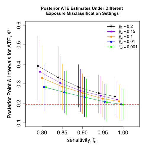
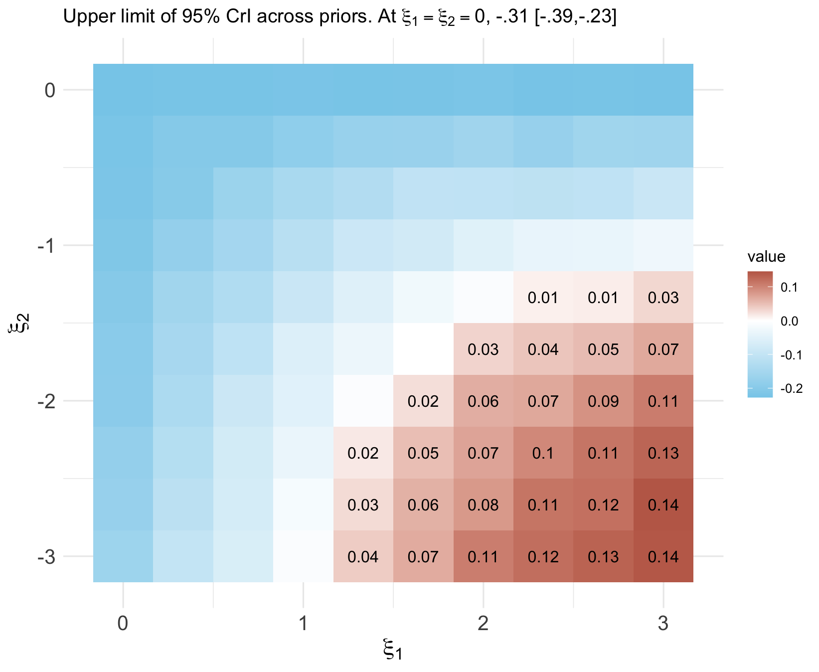
Figure 1: Posterior mean and 95% credible intervals for the ATE under various levels of treatment misclassification, with critical “tipping point” quantification.

Marginalization over the discrete latent indicators is performed analytically to yield a Stan-computable mixture log-likelihood. Results demonstrate nontrivial sensitivity: with increased misclassification (lower $\xi_1$, higher $\xi_2$), ATE credible intervals expand and may cross the null, illustrating potential bias magnitude.

Unmeasured Confounding

For sensitivity to unmeasured confounding, an unobserved continuous confounder $U$ is incorporated into outcome and treatment models, each parameterized by nonidentified log-odds coefficients $(\xi_1, \xi_2)$. Priors are fixed at null or alternative values, reflecting varying beliefs about plausible confounder effects. Stan implementation is straightforward since latent $U$ is continuous, allowing full Bayesian posterior simulation.

Notably, results illustrate that modest deviations from unconfoundedness (in plausible E-value ranges) can materially alter inferences, often shifting credible intervals to include or exclude null effects—a phenomenon immediately readable from “tipping point” analyses.

Missing Not-at-Random Outcomes

For MNAR scenarios, the missingness mechanism is explicitly modeled as a function of latent outcome, observed treatment, and covariates, governed by sensitivity parameters. Inclusion of outcome in the missingness regression (logistic or otherwise) induces dependence that violates missing-at-random (MAR), necessitating bespoke Bayesian inference. Because Stan does not allow discrete parameters in the sampling block, the paper details analytical marginalization over missing outcomes for the observed data likelihood and mixture-based coding of the posterior.

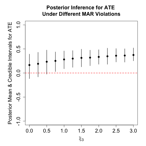
Figure 2: Sensitivity of the ATE to increasing deviations from MAR in the outcome missingness mechanism; credible intervals crossing the null reflect increased sensitivity.

Applied examples show that for datasets with high proportions of missing outcomes, even moderate MNAR deviations rapidly shift posterior inference, emphasizing the practical necessity of explicit sensitivity quantification.

Bayesian Nonparametric Sensitivity Analyses

To address model flexibility and overcome parametric constraints, the paper demonstrates application of truncated stick-breaking (TSB) mixtures as nonparametric priors over the full data-generative process. The mixture induces highly adaptive outcome and covariate regression functions, with the unidentifiable aspects (missingness, misclassification, unmeasured confounding) still captured by explicit, lower-dimensional sensitivity parameters.

When fitting TSB models in Stan, mixture weights are parameterized via Beta priors (stick-breaking process), and standardization for the ATE is performed over the fitted mixture. This approach allows regions of the parameter space with observed data to inform the mixture-driven regression, while inference in unobserved regions is necessarily governed by the sensitivity parameter priors.

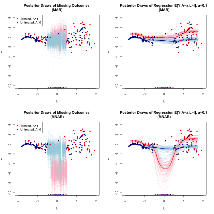
Figure 3: Posterior inference for MNAR outcomes using TSB mixtures, demonstrating shifts in pointwise posterior distributions of missing outcomes and treatment regression lines as MNAR sensitivity parameters are modified.

Practical and Theoretical Implications

The guide underscores several advantages and challenges for practical researchers:

• Bayesian sensitivity analysis, especially in Stan, gives direct control over encoding subject-matter assumptions and expert beliefs regarding assumption violations.
• Utilization of flexible nonparametric models, coupled with explicit sensitivity parameters, bridges the gap between robust model fitting and bias analysis.
• Implementation is feasible with public software, provided care is taken with the necessary marginalizations and custom log-likelihoods.
• Tipping point analyses illuminate the robustness or fragility of causal inferences, which is critical for transparent reporting and policy translation.

On the theoretical level, the framework demonstrates that Bayesian inference unifies parameter and missing data estimation and makes clear the precise location and magnitude of “ignorability gaps.” Sensitivity analysis becomes an explicit part of inference rather than an afterthought or post hoc critique.

Future Directions and Outlook

Opportunities for extension include developing more sophisticated priors over sensitivity parameters (beyond point mass), integrating external validation data, and expanding to longitudinal/complex treatment regimes (e.g., dynamic treatment regimes with time-varying confounding and measurement error). Furthermore, increased automation of the analytical marginalization steps and enhanced computational strategies for high-dimensional or non-discrete missing data can further broaden access.

Conclusion

This work synthesizes and operationalizes Bayesian sensitivity analysis for a range of causal inference problems, providing methodological clarity, detailed implementation advice, and vivid empirical illustrations. By mapping inference under assumption violation to Bayesian missing data modeling, and exploiting Stan’s programmability, robust causal effect estimation—accounting for both structural and statistical uncertainty—becomes tractable and transparent. The approach is poised for broader adoption in applied biomedical research, contingent upon expanded practitioner familiarity with both theoretical grounding and practical modeling skills.