Weak Diffusion Priors Can Still Achieve Strong Inverse-Problem Performance
Abstract: Can a diffusion model trained on bedrooms recover human faces? Diffusion models are widely used as priors for inverse problems, but standard approaches usually assume a high-fidelity model trained on data that closely match the unknown signal. In practice, one often must use a mismatched or low-fidelity diffusion prior. Surprisingly, these weak priors often perform nearly as well as full-strength, in-domain baselines. We study when and why inverse solvers are robust to weak diffusion priors. Through extensive experiments, we find that weak priors succeed when measurements are highly informative (e.g., many observed pixels), and we identify regimes where they fail. Our theory, based on Bayesian consistency, gives conditions under which high-dimensional measurements make the posterior concentrate near the true signal. These results provide a principled justification on when weak diffusion priors can be used reliably.
Paper Prompts
Sign up for free to create and run prompts on this paper using GPT-5.
Top Community Prompts
Explain it Like I'm 14
Clear, simple explanation of “Weak Diffusion Priors Can Still Achieve Strong Inverse-Problem Performance”
1) What is this paper about?
This paper asks a surprising question: do you really need a super-accurate image generator to fix a damaged photo? The authors show that even “weak” diffusion models—generators that are low-quality or trained on a different kind of images—can still help you recover good images in many cases. They explain when this happens, why it happens, and where it fails.
Think of it like fixing a jigsaw puzzle with some missing pieces. If you can still see most of the picture, you don’t need to be an expert on that exact kind of puzzle—you can still put it together. But if most of the picture is gone, you need a lot more prior knowledge to fill in the gaps.
2) What questions did the paper ask?
In plain terms, the paper explores:
- Can a weak or mismatched image generator (like one trained on bedrooms) help reconstruct a different kind of image (like a human face)?
- When do the measurements (the pixels you can still see) give so much information that they outweigh the generator’s weaknesses?
- When do weak generators fail, and why?
- Can we design simple, stable methods to use weak generators effectively?
3) How did they approach it?
The authors used both experiments and theory.
- What is a “diffusion prior”?
- A “strong” prior: a full, high-quality diffusion model trained on the same kind of images you want to reconstruct.
- A “weak” prior: a few-step generator (blurry, low-detail) and/or a model trained on a different dataset (mismatch).
- What is the task? An inverse problem is like fixing a corrupted image: inpainting (filling in masked pixels), deblurring, or super-resolution (recovering a high-res image from a low-res one). You have a measurement (the damaged/partial picture) and you want to recover the original image.
- Their simple solve strategy: adjust the seed noise.
- AdamSphere: a version of a standard optimizer (Adam) that keeps the seed on the “usual size” sphere. In high dimensions, typical random seeds lie on a shell of a certain radius; staying there keeps generation stable.
- HoldoutTopK early stopping: they set aside some measurements as a mini “validation set” and stop when performance on that set is among the best K times. This helps avoid overfitting noise.
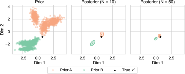
- Their theory in everyday words: They show that if your measurements contain a lot of information (for example, many pixels are visible), then the data can “overpower” the prior. In Bayesian terms, the posterior (your updated belief after seeing data) concentrates near the true image even if your initial prior was not perfect. To make this analyzable, they model the generator’s “prior” as a mixture of simple shapes (think: a bag of prototypical images plus small noise). When many pixels are observed, the “best-matching prototype” stands out clearly, and the math shows the posterior will overwhelmingly choose it. In short: more observed pixels → less need for a perfect prior.
4) What did they find, and why is it important?
Here are the main results the authors report:
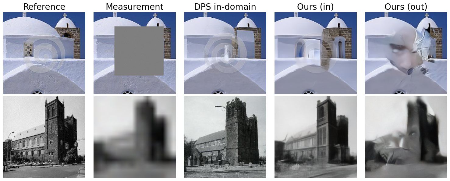
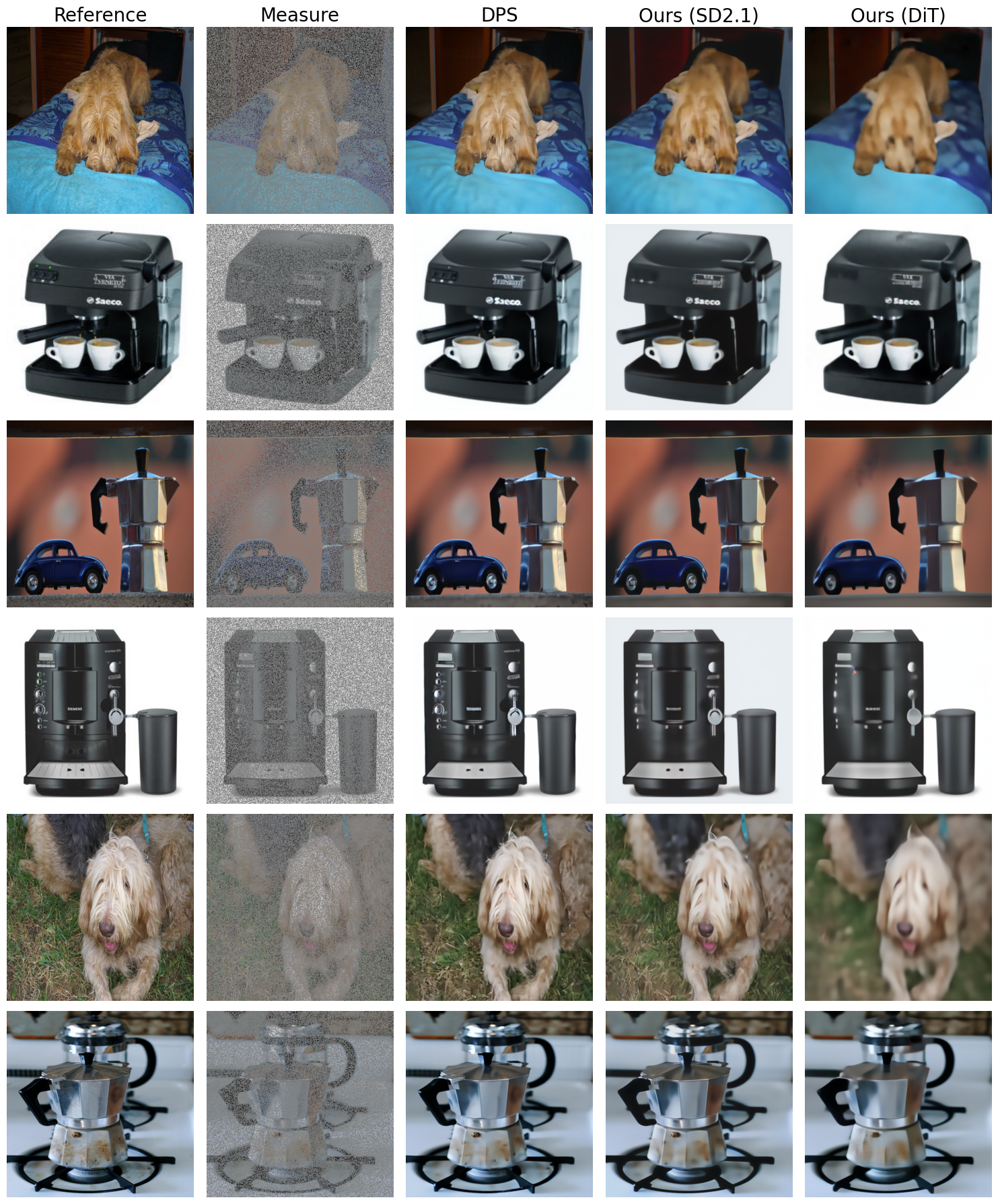
- Weak priors often work well when the data is informative. In tasks like random inpainting (lots of pixels observed) or moderate super-resolution, even a 3-step, low-fidelity generator can reconstruct images competitively, sometimes matching or beating a strong baseline that uses a full diffusion model.
- Cross-domain success is possible. A generator trained on bedrooms can help reconstruct faces—and vice versa—when enough pixels are observed. The differences matter, but less than you’d expect when the measurements are strong.
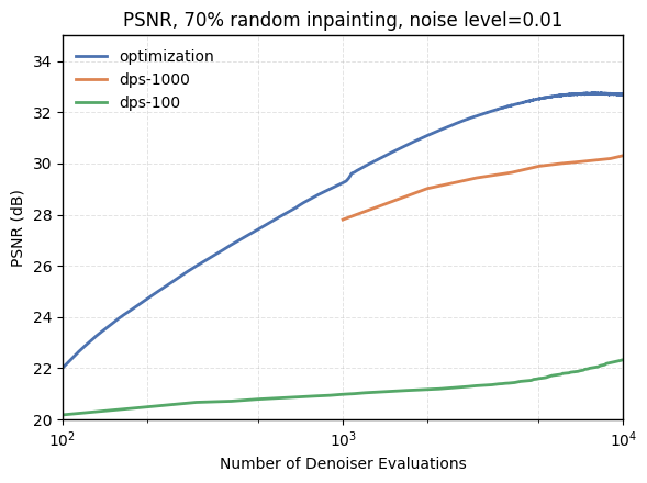
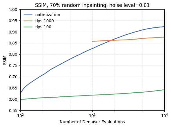
- Their simple optimizer and early stopping help. The AdamSphere optimizer keeps seeds in a stable range; the HoldoutTopK stopping method avoids overfitting to noise. Together, they outperform or match a strong optimization-based baseline (DMPlug) on several tasks in PSNR/SSIM and perceptual quality (LPIPS).
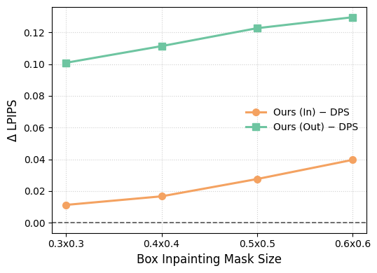
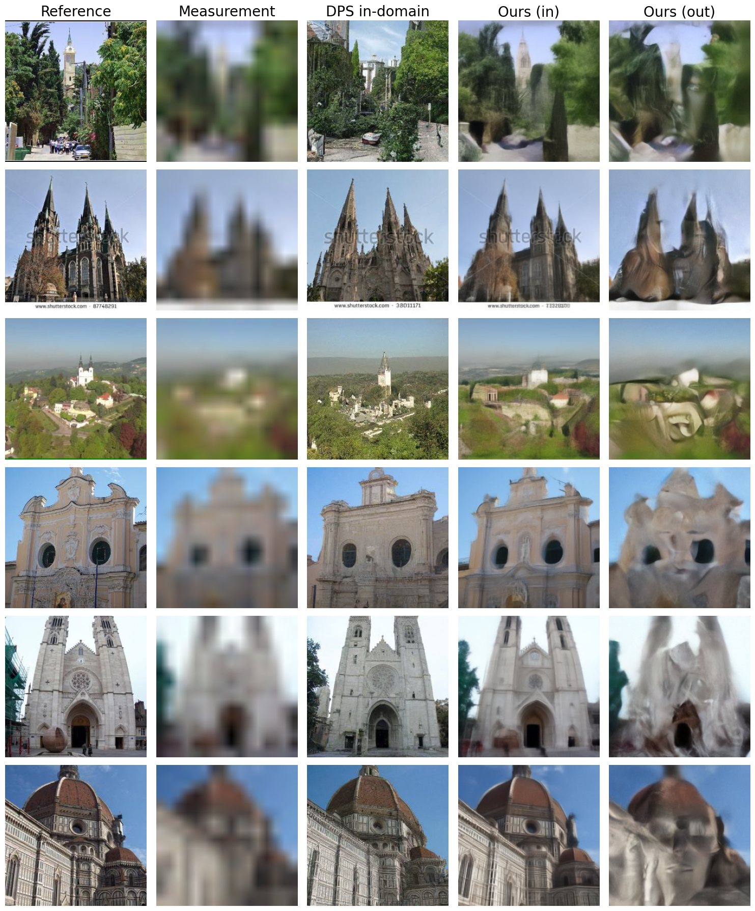
- There are clear failure modes.
- Box inpainting with a big missing square (you must “imagine” a whole region), or
- Very large super-resolution (like 16×, where little information remains)—
- weak priors often fail, and stronger in-domain diffusion models do better. In these cases, you need strong prior knowledge to fill in the gaps.
- The theory backs up the experiments. The authors prove that when many measurements are available and the “best match” stands out, the posterior will concentrate around the correct image—roughly, the data “washes out” the prior. When few measurements are available, the prior matters much more.
Why it matters: this means you may not need a perfect, giant, domain-specific diffusion model to get strong results—especially when your measurements contain a lot of information. That can save time, compute, and reduce the need for hard-to-get training data.
5) What’s the impact of this research?
- Practical takeaway: if you must work with limited compute, memory, or mismatched training data, don’t give up. A weak or out-of-domain diffusion model—used with smart optimization and early stopping—can still produce strong reconstructions when you observe enough of the image.
- When to be careful: if huge areas are missing or the task throws away a lot of information, weak priors will likely struggle. In those cases, a strong, well-matched prior is still important.
- Bigger picture: the work encourages the community to:
- Build and study methods tailored to few-step, weak priors.
- Combine “injecting measurements” and “seed optimization” for the best of both worlds.
- Develop better ways to detect when measurements are informative enough, and when they aren’t.
In short, this paper tells a hopeful and practical story: when you have good clues, even a rough helper can guide you home. When clues are scarce, bring a stronger guide.
Knowledge Gaps
Knowledge gaps, limitations, and open questions
The paper establishes when weak diffusion priors can perform well and presents supporting experiments, but several aspects remain unresolved or underexplored. The following concrete gaps could guide future research:
- Precise data-informativeness thresholds: Derive necessary and sufficient conditions for prior-robustness in terms of measurement dimension , noise level , spectrum and structure of , and mask topology (random vs. contiguous), including sharp constants for the exponential concentration rate.
- Beyond Gaussian-mixture surrogates: Prove posterior concentration for realistic diffusion priors (score-based or DDIM/DDPM samplers) without the finite, isotropic Gaussian-mixture approximation; relax bounded-weight-ratio and equal-variance assumptions; treat heteroscedastic, anisotropic, or heavy-tailed components and infinite mixtures.
- Continuous-manifold priors: Replace the dependence on a finite component count with bounds based on metric entropy/covering numbers of data manifolds; handle multi-modal or near-symmetric manifolds where unique minimizers may not exist.
- Nonlinear and non-Gaussian measurement models: Extend theory and experiments to nonlinear (e.g., saturation, demosaicing, JPEG), Poisson/shot noise and heteroscedastic noise, and physics-based operators (MRI Fourier, CT/Radon), including model misspecification.
- Failure boundary mapping: Quantify the transition from data-dominated to prior-dominated regimes for structured masks (box inpainting) and large-factor super-resolution; characterize how , , operator conditioning, and downsampling factors jointly determine failure.
- Practical diagnostics of informativeness: Develop per-instance tests/estimators for effective observed dimensionality and the identifiability gap (or proxies) computable from to predict when weak priors are safe to use.
- Empirical validation of identifiability: Move beyond dataset-wide nearest-neighbor MSE gaps to candidate sets induced by the actual generator; study dependence of gap statistics on noise level, mask pattern, and resolution with uncertainty quantification.
- Prior mismatch quantification: Define operational measures of source–target mismatch (e.g., CLIP/FID/feature distances) and map reconstruction quality as a continuous function of mismatch; identify thresholds where performance degrades.
- Optimization landscape analysis: Theoretically analyze the nonconvex objective for few-step generators—conditions for reaching the correct posterior mode, effects of non-injective , initialization, and benefits of multi-start or diversity-promoting strategies.
- AdamSphere and HoldoutTopK guarantees: Provide theory for convergence and generalization, guidance on sphere radius, holdout fraction, and ; quantify data-efficiency loss from holding out measurements and robustness under high noise or ill-conditioned .
- Uncertainty quantification: Extend beyond point estimates to posterior sampling or calibrated ensembles under weak priors; assess calibration and coverage, especially under domain mismatch.
- Compute–quality scaling laws: Establish scaling relationships between number of DDIM steps, optimization iterations, and error; provide compute-matched comparisons to DPS and other baselines across budgets, including energy/memory profiles.
- Broader baselines and tasks: Benchmark against additional strong-prior and plug-and-play methods (e.g., DDRM, DDNM, PnP/RED, DRUNet) and tasks (blind SR, compressed sensing, deconvolution, dehazing), including scientific/medical imaging with realistic forward models.
- Latent diffusion specifics: Analyze interactions between pixel-space and latent-space priors (autoencoder distortion, decoder Jacobians); evaluate across more ImageNet classes and conditioning types; study how conditioning (e.g., text prompts) affects weak-prior robustness.
- Robustness to forward-model and noise misspecification: Quantify sensitivity to errors in , misestimated , and systematic/artifact corruption; develop robust objectives or estimators to mitigate misspecification.
- Hybrid algorithms: Design and evaluate methods that combine measurement injection (DPS-style) with latent optimization for few-step priors; study schedules, stability, and theoretical impacts on posterior concentration.
- Choosing the number of sampling steps: Systematically chart performance vs. DDIM step count (1–10+) across tasks and datasets; identify minimal that preserves prior-robustness and the regimes where further steps materially help.
- Seed sensitivity and reproducibility: Quantify variance across random initializations and benefits of averaging, selection, or deterministic initializations; report confidence intervals for metrics.
- Ethical and failure-aware deployment: In prior-dominated regimes, weak priors may hallucinate semantically incorrect content; develop detection mechanisms, user-facing uncertainty reporting, and safeguards for safety-critical domains.
- Early-stopping selection effects: Assess whether HoldoutTopK introduces selection bias; compare with alternative holdout/cross-validation strategies and study their statistical properties.
- Multi-observation settings: Extend theory from single high-dimensional observations to multiple low-dimensional views; connect i.i.d. posterior consistency with high-dimensional single-observation results and identify trade-offs.
- Generalization to alternative priors: Test and analyze whether robustness extends to flows, autoregressive models, and VAEs; identify prior properties (e.g., Lipschitzness, smoothness) that enable weak-prior success.
- Real-world sensor constraints: Evaluate effects of quantization, color space conversions, HDR ranges, and device-specific noise on weak-prior robustness and algorithm stability.
Practical Applications
Immediate Applications
Below are concrete, deployable use cases that leverage the paper’s findings that weak/mismatched diffusion priors (e.g., few-step DDIM/latent diffusion) can still perform strongly when measurements are informative, together with the proposed AdamSphere optimizer and HoldoutTopK early stopping.
- Edge/device-friendly image restoration for consumer and enterprise cameras — software, mobile, media
- Use cases: smartphone camera pipelines, bodycams/dashcams, drones, AR/VR headsets, surveillance video remediation (denoising, deblurring, deartifacting, 2–4× super-resolution), old photo enhancement.
- Tools/products/workflows: integrate a few-step diffusion prior and initial-noise optimization with
AdamSphere+HoldoutTopKas a drop-in “inverse plug-in” in ISP/vision stacks; expose a “weak-prior mode” to reduce latency and power. - Assumptions/dependencies: differentiable/known forward operator A (e.g., blur kernel, downsampler), good noise estimation, sufficiently many observed pixels (data-informative regime), moderate super-resolution factors (≤4×), avoidance of large contiguous missing regions.
- Cross-domain medical image reconstruction when in-domain models are unavailable — healthcare
- Use cases: low-dose CT denoising, sparse-view CT, MRI inpainting/deblurring, out-of-distribution scans (e.g., using a brain-MRI prior on knee MRI).
- Tools/products/workflows: a reconstruction module that defaults to weak or mismatched priors (e.g., general latent diffusion) plus
AdamSphereandHoldoutTopKto control overfitting; routing logic that chooses weak-prior mode when no matched prior exists. - Assumptions/dependencies: ample measurement information (e.g., sufficient k-space lines or projection angles), calibrated noise level, documented forward model, clinical validation and regulatory QA; failure expected in very sparse or large-hole regimes.
- Industrial inspection and non-destructive testing (NDT) — manufacturing, aerospace, automotive
- Use cases: X-ray/ultrasound deblurring/denoising for defect detection when domain-specific priors are scarce.
- Tools/products/workflows: on-line inspection pipeline with weak-prior inverse solver and
HoldoutTopKto avoid fitting sensor noise; fallback to weak-prior mode during model cold-starts. - Assumptions/dependencies: accurate forward model (e.g., PSF), sufficient SNR and measurement coverage.
- Remote sensing and Earth observation — geospatial, energy, climate
- Use cases: satellite/aerial image deblurring, moderate super-resolution (2–4×), random-mask inpainting (e.g., partial cloud occlusions).
- Tools/products/workflows: GIS plugin for batch reconstruction using few-step priors; job scheduler that toggles strong vs. weak prior based on coverage/occlusion statistics.
- Assumptions/dependencies: avoid large contiguous missing blocks; sensor model known; measurement dimension high (many pixels).
- Computational microscopy and scientific imaging — life sciences, materials
- Use cases: fluorescence deconvolution, denoising under photon-limited settings when domain priors are weak or mismatched.
- Tools/products/workflows: pipeline replacement of heavy reverse-diffusion solvers with few-step generators + latent optimization; validation using held-out measurement subsets.
- Assumptions/dependencies: known PSF, data-informative acquisition; quantitative validation for downstream analysis.
- Cost and energy reduction in cloud inference — software platforms
- Use cases: large-scale restoration services (e.g., photo/video enhancement) reduce compute by replacing 50–1000-step solvers with 3–10-step weak priors in data-informative cases.
- Tools/products/workflows: “weak-prior accelerator” mode, dynamic policy that switches to strong priors only when informativeness tests fail (e.g., low m or large box-missingness).
- Assumptions/dependencies: on-line informativeness diagnostic; monitoring to detect failure modes.
- Robust inverse-problem benchmarking and curriculum — academia
- Use cases: standardized evaluation under prior mismatch and truncation; teaching modules on Bayesian consistency and identifiability.
- Tools/products/workflows: open-source baselines implementing
AdamSphere,HoldoutTopK, and cross-domain tests; datasets with predefined measurement holdouts. - Assumptions/dependencies: reproducible access to forward models and noise parameters.
- Procurement and governance checklists emphasizing measurement informativeness — policy
- Use cases: public-sector imaging systems (medical, remote sensing) that cannot train matched priors; policy guidance to prioritize data-informative sensing over model matching.
- Tools/products/workflows: measurement-design checklists (coverage, SNR), documentation of identifiability conditions; QA using held-out measurements.
- Assumptions/dependencies: ability to quantify informativeness (e.g., fraction observed, SNR), risk controls when outside the guaranteed regime.
Long-Term Applications
These applications require further research, scaling, validation, or engineering to fully realize.
- Sensing and measurement design to maximize identifiability — hardware–software co-design
- Use cases: optimize masks/trajectories/k-space sampling to increase the per-dimension score gap δ0 so the posterior concentrates despite weak priors.
- Tools/products/workflows: “A–prior co-design” toolkit that simulates δ0 under candidate sensing patterns; active sensing that adapts measurements on-the-fly.
- Assumptions/dependencies: control over sensing hardware; reliable proxies for δ0; multi-objective trade-offs (dose, speed, resolution).
- Foundation diffusion priors for inverse problems — general-purpose priors
- Use cases: broad latent diffusion models (e.g., SD/DiT-scale) as default priors that perform robustly across domains with informative measurements.
- Tools/products/workflows: hosted “foundation prior service” with APIs for inverse operators; curated adapters for common A (blur, downsample, projection).
- Assumptions/dependencies: large-scale training, safety and bias audits; continued evidence of cross-domain robustness.
- Hybrid solvers that combine DPS-style measurement injection with latent optimization — software, robotics, healthcare
- Use cases: bridge regimes from highly informative (latent optimization excels) to less informative (strong guidance needed).
- Tools/products/workflows: switchable pipelines that interleave guidance and noise optimization; auto-tuners for guidance strength and number of steps.
- Assumptions/dependencies: stability under hybrid updates; compute–quality tradeoff exploration.
- Instance-level reliability and uncertainty quantification — risk management
- Use cases: per-image diagnostics estimating when weak priors are safe (e.g., proxies for δ0 or the MSE score gap), confidence intervals for reconstructions.
- Tools/products/workflows: runtime monitors that flag low-informativeness cases; abstain/route-to-strong-prior policies; audit logs.
- Assumptions/dependencies: calibrated likelihoods, robust score-gap estimators; acceptance criteria for high-stakes domains.
- Extreme generation-heavy regimes (large box inpainting, 8–16× super-resolution) — media, restoration
- Use cases: fill large missing regions or perform very high upscaling with semantic fidelity.
- Tools/products/workflows: condition with strong priors (full-step diffusion, text/image conditioning), retrieval-augmented priors, or domain-specific training.
- Assumptions/dependencies: availability of strong in-domain priors or auxiliary modalities; increased compute budgets; acceptance of generative ambiguity.
- Hardware acceleration for few-step diffusion priors on edge devices — semiconductors, mobile
- Use cases: real-time inverse problems on cameras, wearables, autonomous platforms.
- Tools/products/workflows: kernel-level acceleration for 3–10 diffusion steps and backprop through A; energy-aware schedulers.
- Assumptions/dependencies: specialized AI DSP/NPU support; co-design with imaging pipelines.
- Regulatory-grade validation and standards for prior robustness — healthcare, public sector
- Use cases: certifiable workflows that document robustness to prior mismatch when measurement conditions are met.
- Tools/products/workflows: validation protocols that stress-test informativeness thresholds; reporting standards for A, σ, and early-stopping criteria.
- Assumptions/dependencies: consensus metrics, clinical studies, alignment with regulatory bodies.
- Multimodal and knowledge-guided inverse problems — cross-modal AI
- Use cases: use language/CAD/physics priors to guide reconstruction when data are less informative.
- Tools/products/workflows: prompt-guided inverse solvers; physics-informed priors; retrieval from domain libraries to improve identifiability.
- Assumptions/dependencies: aligned multimodal datasets; safe prompt handling; verification against measurements.
- Extension beyond images — audio, communications, geophysics, energy
- Use cases: speech denoising/de-reverberation, channel estimation, seismic deconvolution/inversion, subsurface imaging with sparse arrays.
- Tools/products/workflows: domain-specific forward operators coupled with few-step priors; holdout-measurement early stopping.
- Assumptions/dependencies: differentiable, accurate A; sufficient measurement dimensionality; domain-specific validation.
- Auto-prior selection and adaptation — MLOps
- Use cases: automatically choose a weak prior (domain/source model, number of steps) based on measured informativeness and budget.
- Tools/products/workflows: “AutoPrior” controller that predicts success with weak priors, triggers stronger priors only when needed.
- Assumptions/dependencies: meta-models predicting failure modes; monitoring and rollback mechanisms.
Cross-cutting assumptions and dependencies
- Data-informative regime: high-dimensional measurements, sufficient coverage, and uniqueness/δ0-identifiability; weak priors degrade in large contiguous holes and very low information (e.g., 16× SR).
- Accurate forward operator and noise model: known or well-estimated A and σ; differentiability to enable backprop.
- Overfitting control: use of
HoldoutTopKor equivalent; access to holdout measurements. - Compute and memory: few-step generators substantially reduce costs; strong priors still needed for generation-heavy tasks.
- Ethical, legal, and regulatory: domain-appropriate validation, especially in safety-critical applications; transparency about prior mismatch and uncertainty.
Glossary
- AdamSphere: A modified Adam optimizer that constrains the latent noise to remain on a fixed-radius sphere during optimization to prevent degenerate solutions. "We therefore propose AdamSphere, a modified Adam optimizer that keeps on the sphere throughout."
- Bayesian consistency: A property ensuring that as data become sufficiently informative, the posterior distribution concentrates near the true parameter regardless of the prior. "Our theory, based on Bayesian consistency, gives conditions under which high-dimensional measurements make the posterior concentrate near the true signal."
- Box inpainting: An inpainting setup where a contiguous rectangular region of the image is missing, making the problem highly underdetermined. "Firstly, in large box inpainting (where masks a contiguous block), many images can match the observed pixels closely while differing a lot inside the missing box."
- Categorical random variable: A discrete random variable that takes one of a finite set of categories with specified probabilities. "Let be a categorical random variable on with $\bP(J=j) := \tilde w_j/(\sum_{i=1}^M \tilde w_i),$"
- DDIM (Denoising Diffusion Implicit Models): A deterministic sampling procedure for diffusion models that enables faster generation with fewer steps. "Image reconstruction using only a 3-step DDIM generator as the prior: matched prior (top) vs. mismatched prior (bottom)."
- DDPM (Denoising Diffusion Probabilistic Models): A probabilistic diffusion model framework that gradually denoises from noise to data through many reverse steps. "for example, a $1000$-step DDPM \cite{ho2020denoising, song2020score} trained on a face dataset to recover human faces."
- Data-informative regime: A setting where measurements are sufficiently rich or high-dimensional such that the observation largely determines the solution, reducing sensitivity to the prior. "weak priors can still yield strong results in data-informative regimes, where observations are high-dimensional and the signal is identifiable from the measurements."
- δ0-identifiability: A condition ensuring that the best-scoring candidate under the measurement model is uniquely separated from competitors by at least a constant per-dimension gap. "Under a -identifiability assumption, we show that high-dimensional measurements force the posterior to concentrate at an exponential rate around the true signal."
- Diffusion posterior sampling (DPS): A class of solvers that modify reverse diffusion updates to incorporate measurement likelihoods for inverse problems. "Among them, diffusion posterior sampling (DPS) \cite{chung2023diffusion} is one of the most popular solvers, so we take it as our baseline."
- DMPlug: An optimization-based inversion method that solves inverse problems by directly optimizing the initial noise input to a diffusion generator. "Next, we compare our method with the state-of-the-art optimization-based approach DMPlug \cite{wang2024dmplug}."
- Effective observed dimensionality: A measure of how much independent information an observation provides about the signal, influencing how strongly the data can dominate the prior. "We formalize the information content of an observation through its effective observed dimensionality and the identifiability of the signal from the measurements."
- Forward operator: The mapping from the signal to the measurement space that models the physical acquisition process. "The map $A:\bR^n \to \bR^m$ is called the forward operator,"
- Gaussian mixture: A probabilistic model that represents a distribution as a weighted sum of Gaussian components; used here as a surrogate for generative priors. "we assume the prior is an isotropic Gaussian mixture"
- Guidance (in diffusion models): A technique to steer diffusion sampling toward satisfying measurement constraints or desired attributes. "This adjustment has been implemented in many ways, such as guidance, variable splitting, and sequential Monte Carlo;"
- HoldoutTopK: An early-stopping strategy that selects among the best K iterates based on performance on a held-out subset of measurements to mitigate overfitting. "We propose HoldoutTopK early stopping."
- Inference-time scaling: Increasing inference-time compute or optimization effort to improve results without retraining the model. "initial-noise techniques have recently attracted interest across a range of applications for their potential to support inference-time scaling;"
- Initial-noise optimization: Solving inverse problems by optimizing the latent noise input to a pretrained generator so that its outputs match the observations. "Initial noise optimization: Another line of work treats the generative model as a black-box generator and solves inverse problems by optimizing the latent input."
- Inpainting: An inverse problem where missing pixels are reconstructed from observed pixels and a prior. "The left panel illustrates an inpainting task on a human face"
- Inverse problems: Tasks that aim to recover an unknown signal from indirect or noisy measurements using a forward model and prior information. "Inverse problems aim to recover an unknown signal from noisy measurements."
- Latent diffusion models: Diffusion models that operate in a compressed latent space rather than pixel space, often enabling faster and more scalable inference. "we further evaluate our method using latent diffusion models on ImageNet."
- LPIPS (Learned Perceptual Image Patch Similarity): A perceptual similarity metric that compares deep features of image patches to assess visual similarity. "We evaluate each method using standard metrics, including PSNR, SSIM, and LPIPS \cite{zhang2018unreasonable}."
- MAP estimate (Maximum a Posteriori): The mode of the posterior distribution, representing the most probable signal given data and prior. "or compute the maximum a posteriori (MAP) estimate ."
- Measurement operator: The linear or nonlinear operator that maps a clean signal to its observed measurements, e.g., masking or downsampling. "For inpainting problems, the measurement operator is a coordinate projection"
- Peak Signal-to-Noise Ratio (PSNR): A logarithmic metric (in dB) for measuring reconstruction fidelity relative to signal range and error. "reports a $2$--$6$ dB PSNR improvement over state-of-the-art baselines"
- Per-dimension score gap: The average difference (per observed dimension) between the best and second-best measurement residual scores, controlling posterior concentration. "We define the per-dimension score gap as"
- Posterior collapse: Concentration of the posterior on a single mixture component or mode under strong measurement evidence. "Posterior collapse to the best-scoring mode."
- Posterior consistency: The asymptotic property that the posterior converges to the true parameter as the amount of (i.i.d.) data grows. "This is an instance of posterior consistency."
- Reverse diffusion chain: The sequence of denoising steps that transforms noise into data samples during diffusion model sampling. "by injecting measurement information throughout a reverse diffusion chain to enforce consistency with the observation"
- Sequential Monte Carlo: A set of particle-based inference methods that approximate distributions by evolving weighted samples through a sequence of intermediate targets. "This adjustment has been implemented in many ways, such as guidance, variable splitting, and sequential Monte Carlo;"
- SSIM (Structural Similarity Index Measure): An image quality metric that measures structural similarity between images using luminance, contrast, and structure components. "We evaluate each method using standard metrics, including PSNR, SSIM, and LPIPS"
- Super-resolution: An inverse problem that reconstructs a high-resolution image from its low-resolution observation. "The right panel of Figure~\ref{fig:teaser} shows a super-resolution experiment with similar conclusions."
- Total-variation distance: A metric on probability distributions that measures the maximum difference in probabilities assigned to events. " stands for total-variation distance."
- Variable splitting: An optimization technique that introduces auxiliary variables to decouple complex objectives, often used with alternating updates. "This adjustment has been implemented in many ways, such as guidance, variable splitting, and sequential Monte Carlo;"
- Weak diffusion prior: A diffusion-based prior that is either low-fidelity (e.g., few-step sampler) or trained on a mismatched dataset relative to the target domain. "we study when and why inverse solvers are robust to weak diffusion priors."
Collections
Sign up for free to add this paper to one or more collections.

