Many Experiments, Few Repetitions, Unpaired Data, and Sparse Effects: Is Causal Inference Possible?
Abstract: We study the problem of estimating causal effects under hidden confounding in the following unpaired data setting: we observe some covariates $X$ and an outcome $Y$ under different experimental conditions (environments) but do not observe them jointly; we either observe $X$ or $Y$. Under appropriate regularity conditions, the problem can be cast as an instrumental variable (IV) regression with the environment acting as a (possibly high-dimensional) instrument. When there are many environments but only a few observations per environment, standard two-sample IV estimators fail to be consistent. We propose a GMM-type estimator based on cross-fold sample splitting of the instrument-covariate sample and prove that it is consistent as the number of environments grows but the sample size per environment remains constant. We further extend the method to sparse causal effects via $\ell_1$-regularized estimation and post-selection refitting.

Paper Prompts
Sign up for free to create and run prompts on this paper using GPT-5.
Top Community Prompts
Explain it Like I'm 14
What this paper is about (big picture)
The paper asks a tough question: if you run many different experiments, but in each one you can measure either the input () or the outcome (), never both together, can you still figure out how causes ? Even harder, what if there are hidden confounders (unseen factors) that affect both and ?
Surprisingly, the answer is yes—under reasonable conditions. The authors show when and how this is possible, and they build methods that work well, especially when there are many experiments but only a few measurements per experiment.
What questions the paper answers
The paper focuses on these simple questions:
- If and are never measured together (unpaired data), can we still estimate the causal effect of on ?
- What conditions do we need for this to work, especially when there are hidden confounders?
- What happens when we have many different experimental conditions (or “environments”), but only a few repeats in each one?
- Can we get good estimates even when there are many variables and only a few of them truly matter (sparse effects)?
How the methods work (in everyday language)
Think of each “environment” as one experimental condition (like changing which gene is edited, which lab chemical is used, or which hospital the data comes from). We use the environment as an “instrument”—a special kind of variable that nudges but does not directly push . This is the key idea behind instrumental variables (IV).
Here’s the challenge and the fix, using analogies:
- The challenge: Unpaired data is like having two photo albums of the same vacation—one with pictures of people () and one with pictures of places ()—but no single picture shows a person and a place together. You can’t directly match who was where. Also, hidden confounders are like bad lighting that makes it hard to tell what’s going on.
- The instrumental variable trick: The environment is like a remote control that changes but, by assumption, doesn’t change except through . If the remote only affects , differences across environments help us tease out the true effect of on .
- What goes wrong with standard methods: A common approach is to average within each environment and then regress those averages. That works if each environment has lots of repeats. But when you have many environments and only a few measurements in each, those averages are noisy, and the usual methods become biased.
- The authors’ fix (cross-fold “two-camera” idea): They split the -data across folds and compare “cross-moments” (think: combining independent views), which cancels out the main measurement-error bias. This idea makes their estimator consistent—that is, it gets closer to the truth as you add more environments—even if each environment has only a few measurements.
- Handling many ’s when only a few matter (sparse effects): They use an penalty (also called Lasso) that encourages a simple model, picking out the few ’s that actually affect . After selecting these, they refit without the penalty to get cleaner estimates and confidence intervals.
In slightly more technical but still friendly terms:
- They show when the causal effect vector is identifiable from the joint behavior of (environment, ) and (environment, ), even though and aren’t paired.
- For many environments (“high-dimensional instruments”), they define a limit matrix that captures how environments move . If has enough “variety,” the causal effect is uniquely determined.
- For sparse effects, they need weaker conditions: roughly, you don’t need environments to span all directions of , only those that matter.
What they found and why it’s important
Here are the main takeaways:
- Unpaired data can still give valid causal estimates. If environments affect but not directly (the IV assumption), you can identify the causal effect of on from separate samples: one with and one with .
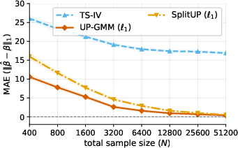
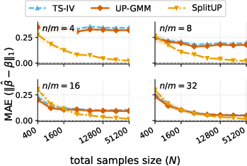
- Standard two-sample IV methods can fail when there are many environments but few repeats per environment. They become biased because the estimated relationships are noisy (“measurement-error bias”).
- The paper introduces a cross-fold, GMM-based estimator that fixes this bias. It stays consistent as the number of environments grows, even if the number of measurements per environment stays small.
- The method extends to sparse effects using an -regularized version (Lasso). It can correctly identify which variables matter and estimate their effects, even when there are more ’s than environments.
- They also provide conditions for when the causal effect is identifiable:
- Dense case (many non-zero effects): you need enough variation from environments to cover all directions of .
- Sparse case (few non-zero effects): you can get away with less variation—roughly, you need enough instruments to distinguish the few active variables.
- After selecting the important ’s, they refit without the penalty and can build valid confidence intervals, giving practical uncertainty estimates.
Why this matters:
- In real biology and medicine, you often can’t measure everything in the same cell or patient at the same time. For example, one experiment may measure gene expression (), another measures a phenotype like growth rate (), and the cells are different—so the data are unpaired. This method makes such studies much more useful for causal questions.
- The results also guide study design: if you can run many different environments, you don’t necessarily need many repeats in each; you just need the environments to move in informative ways.
Practical implications and impact
- Better use of modern experiments: The approach is especially relevant for large-scale biological screens (e.g., CRISPR gene edits, drug treatments) where and are hard to measure together.
- Works with both categorical and continuous environments: The framework handles “environment” as either different categories (like different labs or gene edits) or continuous variables (like dosage).
- Scales to many features: If only a few ’s truly affect , the sparse version can recover them reliably—even when there are more features than instruments.
- Safer estimates: The cross-fold idea reduces bias that plagues standard methods when instruments are many and per-instrument data are few.
- Clear assumptions: The key assumption is the instrumental variable condition: environments affect only through (no direct path). When that holds, the method gives consistent estimates and valid uncertainty.
In short, the paper shows that even with unpaired data, hidden confounders, many environments, and few measurements per environment, causal inference is still possible. With careful design (using environments as instruments) and the right estimator (cross-fold GMM, with optional sparsity), you can get reliable, interpretable causal effects that matter for biology, medicine, economics, and other fields.
Knowledge Gaps
Knowledge gaps, limitations, and open questions
Below is a single, concrete list of what remains missing, uncertain, or unexplored, to guide future research.
- Robustness to violations of Assumption 1 and 1′: quantify bias and derive sensitivity analyses when Cov(I, X) differs across samples and/or exogeneity E[ε | I] ≠ 0 (including small/structured violations).
- Estimation and inference when the two samples are dependent or partially overlapping (contradicting the independence assumed in the estimation section); develop estimators valid under cross-sample dependence.
- Detection and correction for invalid instruments (environments with direct or pleiotropic effects on Y): diagnostics, robust estimators (e.g., MR-Egger–type, mode-based), and identifiability under subsets of valid instruments.
- Causal effect heterogeneity across environments: tests for invariance of β*, models allowing environment-specific or moderated effects, and identification when β varies.
- Finite-sample behavior of the cross-fold (split-sample) GMM estimator: optimal choice of the number of folds K, repeated splitting and aggregation, and analytical/empirical quantification of split-induced variance.
- Asymptotic normality and feasible variance estimation for the high-dimensional cross-moment estimator: explicit CLTs, sandwich covariance formulas, and consistent plug-in estimators for inference.
- Practical estimation of Q and W0 in the high-dimensional regime: stable estimators, conditions ensuring positive definiteness, and procedures for near-singular Q (regularization, ridge-type corrections).
- Weak-instrument diagnostics and valid tests in the unpaired, high-dimensional setting (analogs of Anderson–Rubin, Kleibergen–K, conditional LR), including critical values and power properties.
- Valid post-selection inference for sparse β* in the high-dimensional instrument regime: debiasing/double selection, confidence intervals for selected coordinates, and control of selection mistakes without beta-min assumptions.
- Practical verification of restricted nullspace/eigenvalue conditions for Cov(I, X) or Q: data-driven diagnostics, bounds, and design criteria that guarantee these conditions.
- Extension and explicit conditions for continuous instruments beyond the categorical example (Assumption hd-weak): illustrative models, sufficient conditions, and empirical checks.
- Within-environment dependence and unequal repetitions per environment: cluster-robust covariance, weighting schemes for varying environment sizes/heteroskedasticity, and associated theory.
- Performance under extreme sample size imbalance (e.g., rare environments, highly skewed instrument distributions), and adjustments to stabilize estimation.
- Methods for combining partially paired data with unpaired samples: hybrid estimators that exploit any available X–Y pairs while retaining unpaired information.
- Measurement error in instruments I and mismeasurement in X or Y: bias characterization and measurement-error–robust estimators in the unpaired IV setting.
- Robustness to heavy tails and outliers: median-of-means or robust GMM/Lasso variants with guarantees in the proposed regimes.
- Extensions beyond linear additive models: nonlinear/semiparametric structural relations, binary or count outcomes, and corresponding moment conditions and identifiability.
- Computational scalability when m (number of environments/instrument dimension) is large (e.g., one-hot encoding): memory-efficient algorithms, streaming/online updates, and complexity analysis.
- Tuning and weighting: principled, data-driven selection of λ and W_N (and W′_N) with stability guarantees; guidance on their impact on bias/variance, especially in high-dimensional instruments.
- Transportability/bridging when Cov(I, X) differs across samples (violating Assumption 1(i)): calibration methods, reweighting, or covariate shift corrections to recover identifiability.
- Multivariate outcomes or multivariate treatments: joint estimation strategies, identifiability conditions, and inference for vector-valued β*.
- Aggregation across multiple unpaired samples/cohorts: multi-sample GMM designs, meta-analytic moment combination, and heterogeneity-aware pooling.
- Efficiency bounds: semiparametric efficiency characterization for β* in unpaired IV, and whether proposed estimators attain (or can be adapted to attain) efficiency.
- Winner’s-curse and instrument-selection bias in the two-sample regime: mitigations (e.g., selection on one fold and estimation on another), theory for selection-induced bias with many instruments.
- Time-varying or longitudinal environments: dynamic instruments, repeated measures, interference across units, and appropriate moment structures.
- Empirical validation in real biological datasets: stress-testing assumptions (exclusion, Cov(I, X) equality), instrument validity diagnostics, and comparisons to existing two-sample IV/MR methods under realistic violations.
Practical Applications
Immediate Applications
The following are concrete, deployable uses of the paper’s methods and findings. Each item lists sectors, what you can do now, likely tools/workflows that could be built, and key assumptions/dependencies that must hold.
- Biotech and Pharma: Causal target discovery from unpaired perturbation data
- Sectors: Healthcare, biotechnology, drug discovery
- What to do: Combine large-scale perturbation (environment) → molecular readouts (I→X) from one experiment with phenotype screens (I→Y) from another, even when measured on different cells. Estimate causal effects of molecular features X on phenotype Y under hidden confounding using the cross-fold GMM estimator; recover a sparse set of drivers via ℓ1-regularized GMM and refit for valid CIs.
- Tools/workflows: Python/R package implementing cross-fold GMM and ℓ1-regularized GMM; pipelines integrated into LIMS or ML platforms for CRISPR/compound screens; post-selection inference reports listing likely targets with confidence intervals.
- Assumptions/dependencies: Exclusion restriction (environments affect Y only via X: E[ε | I]=0); matching instrument–covariate structure across samples (Cov(I,X) same in both samples); many environments (m large) but few reps per environment acceptable; linear, homogeneous effect across environments; independence between instrument–covariate and instrument–outcome samples for estimation; sparse effect and beta-min for support recovery.
- Two-sample IV in economics with many instruments and small cell sizes
- Sectors: Economics, public policy
- What to do: Re-estimate classic two-sample IV designs (e.g., compulsory schooling, age-at-entry, split-sample IV) when instruments are categorical by cohort/region/time and cell counts are small. Replace naive two-sample IV with the paper’s cross-moment GMM to avoid the high-dimensional measurement-error bias; optionally use ℓ1 penalty when regressors are many but effects are sparse.
- Tools/workflows: Stata/R add-in for cross-fold GMM IV; diagnostic that flags when naive two-sample IV is biased because n/m is bounded; turnkey scripts for panel/categorical instruments (one-hot environments).
- Assumptions/dependencies: Valid instrument exogeneity; same Cov(I,X) across samples (or same environment distributions and same E[X|I] across samples); K≥2 folds on the instrument–covariate sample; linear effect; sufficient instrument relevance (Q ≻ 0 in the many-instrument regime).
- Mendelian randomization with individual-level data under unpaired designs
- Sectors: Genetics, epidemiology
- What to do: When genotype–exposure and genotype–outcome data come from different cohorts (unpaired), and many weak instruments (SNPs) are used, apply cross-fold GMM on the genotype–exposure dataset to eliminate measurement-error bias; use ℓ1 regularization if exposures are high-dimensional and sparse.
- Tools/workflows: MR toolkit extension requiring individual-level exposure data to enable fold-splitting; robust CI via post-selection refit.
- Assumptions/dependencies: Individual-level instrument–exposure data must be available (beyond summary stats) to support cross-fold moments; standard MR exogeneity (no direct paths/pleiotropy) or explicitly acknowledged; harmonized allele coding across samples; linear homogeneous effect; independence across cohorts for estimation.
- Privacy- or platform-constrained A/B/n testing with unpaired logging
- Sectors: Software/product analytics, advertising
- What to do: Estimate causal effects of treatments/features (X) on outcomes (Y) when privacy/technical constraints split feature logging and outcome logging across systems, but assignment or environment indicators (I) are shared. Use cross-fold GMM to remain consistent with many variants/environments and few observations per variant.
- Tools/workflows: Analytics library for experimentation platforms; automated environment one-hot encoding and cross-fold covariance computation; integration into MLOps dashboards.
- Assumptions/dependencies: Consistent environment identifiers across datasets; exclusion restriction (assignment affects Y only via X); linear effect stability across environments; independence between the two samples.
- Industrial quality and operations analytics with unpaired data sources
- Sectors: Manufacturing, IoT/industry 4.0
- What to do: When sensor covariates X (from one data system) and product quality Y (from a different data system) are unpaired but share production line/time-bucket environments I, infer causal effects of process variables on quality. Use ℓ1-regularized cross-fold GMM to identify a small set of levers.
- Tools/workflows: Factory analytics modules that align environment codes, run cross-fold GMM, and generate prioritized control-variable lists with uncertainty.
- Assumptions/dependencies: Reliable environment coding alignment; exogeneity of environments (e.g., scheduled settings changes that do not directly affect Y except via X); linearity; enough environments or regimes.
- Methodological upgrades to existing two-sample IV workflows
- Sectors: Academia, applied stats across domains
- What to do: Replace naive TS-IV in high-dimensional instrument settings with the cross-fold GMM estimator to remove asymptotic attenuation bias; add ℓ1 penalty and post-selection refit when d > m but effects are sparse; compute oracle-like CIs on the selected support.
- Tools/workflows: R/Python implementations exposing: folding, CXX/CXY construction, weight selection (Ω-hat), tuning via cross-validation, and post-selection inference; checklists for identifiability (rank or restricted nullspace in finite m; Q ≻ 0 in m→∞).
- Assumptions/dependencies: As above; careful centering/harmonization; instrument relevance diagnostics; K≥2 folds.
- Data collection and design guidance for many-environment studies
- Sectors: Experimental design in biology, economics, social science
- What to do: Favor breadth (more environments m) over depth (more reps per environment) when pairing is infeasible; ensure the same environment distribution and conditional means across samples; store the environment indicator with consistent encoding to enable IV-style identification.
- Tools/workflows: Design calculators that evaluate identifiability (restricted nullspace or Q), sample-size guidance for m vs n, and diagnostics for exogeneity plausibility.
- Assumptions/dependencies: Ability to control or verify matching of environment distributions; pre-specification of environment coding and logging standards.
Long-Term Applications
These uses require additional research, data availability, or engineering before becoming routine.
- Robust causal estimation under partial instrument invalidity and pleiotropy
- Sectors: Genetics (MR), econometrics, policy evaluation
- Vision: Extend cross-fold GMM to handle mixtures of valid/invalid instruments (direct paths, pleiotropy) via robust GMM, mode/mixture models, or sparse invalid-instrument selection.
- Dependencies: New theory for robustness in unpaired high-dimensional instrument settings; sensitivity analyses; instrument screening protocols.
- Nonlinear and heterogeneous effect extensions
- Sectors: Healthcare, social science, advertising, manufacturing
- Vision: Kernelized or deep GMM with cross-moments; effect heterogeneity across environments; nonparametric identification with unpaired samples.
- Dependencies: Theory and computation for cross-fitted nonlinear moments; identifiability under effect modification by I; scalable optimization and valid inference.
- Federated and privacy-preserving unpaired causal inference
- Sectors: Healthcare (EHR), finance, tech platforms
- Vision: Apply cross-fold strategies within federated learning or secure aggregation so that raw-level instrument–exposure data never leave the data holder, while enabling unbiased cross-moment estimation.
- Dependencies: Cryptographic protocols for cross-moment computation; DP/noise-aware GMM; assessment of privacy–accuracy tradeoffs; governance frameworks.
- End-to-end pipelines for translational medicine (lab-to-clinic linking)
- Sectors: Precision medicine, oncology
- Vision: Combine lab cell-line perturbation data (I→X) with clinical treatment outcomes (I→Y) to prioritize biomarkers and interventions; integrate ℓ1 selection to deliver succinct, actionable signatures for clinical trials.
- Dependencies: Harmonized environment mapping across lab and clinic, confounding-aware design, extensive validation; regulatory-grade software and QA; prospective evaluation.
- Adaptive experiment design to satisfy identifiability and sparsity conditions
- Sectors: Biology, online experimentation, operations
- Vision: Actively choose environments/interventions to improve restricted nullspace properties (finite m) or increase Q’s smallest eigenvalue (many-instrument regime), maximizing power for sparse effect recovery.
- Dependencies: Online/sequential design algorithms; theoretical guarantees under unpaired sampling; simulation frameworks.
- Summary-statistics–only variants for MR and economics
- Sectors: Genetics, macro/microeconomics
- Vision: Adapt cross-moment ideas to settings where only summary associations are available (no fold-splitting possible), via synthetic folds, external reference panels, or bias-correction formulas.
- Dependencies: New estimators for measurement-error correction without individual-level data; calibration using LD/reference panels in MR; careful modeling of sample overlap.
- Domain-specific products embedding the estimator
- Sectors: Biotech platforms, experimentation SaaS, industrial analytics
- Vision: Commercial tools that: ingest unpaired datasets keyed by environments; implement cross-fold GMM (dense/sparse); provide diagnostics (exogeneity, relevance, n/m regime), and deliver decision reports with post-selection CIs.
- Dependencies: Engineering for scale and reliability; UX for diagnostics and assumptions; customer data-model harmonization; ongoing method updates.
- Policy analytics at administrative-data scale
- Sectors: Education, labor, public health
- Vision: Use many cohorts/regions/time environments when exposures and outcomes are siloed across administrative systems; quantify effects with valid post-selection inference for transparency.
- Dependencies: Inter-agency data harmonization of environment identifiers; legal data-sharing pathways; audits for instrument exogeneity; capacity building in statistical teams.
Notes on key assumptions shared across applications:
- Instrument exogeneity/exclusion: E[ε | I] = 0 (environments affect Y only via X).
- Cross-sample alignment: Cov(I,X) must match across samples (achievable if environment distributions match and E[X|I] is the same across samples).
- Instrument relevance: In finite m, rank(Cov(I,X)) (dense) or restricted nullspace (sparse); in many-instrument regime, Q = lim m Cov(I,X)ᵀCov(I,X) exists and is positive definite (or satisfies sparse RE).
- Estimation requirements: Independence between instrument–covariate and instrument–outcome samples for the provided asymptotics; K ≥ 2 folds on the instrument–covariate sample; centering/harmonization; linear, homogeneous causal effect across environments.
- Sparse recovery: ℓ1 methods need sparsity and a beta-min threshold for consistent support selection; post-selection refit provides valid CIs on the selected support.
Glossary
- Anderson–Rubin: A weak-instrument robust test used in instrumental-variable settings to provide valid inference even when instruments are weak. "Anderson--Rubin, Kleibergen--, and conditional likelihood ratio-type tests"
- Asymptotic normality: A large-sample property where an estimator’s distribution approaches a normal distribution as sample size grows. "asymptotically normal."
- Attenuation bias: Bias toward zero that arises when regressors are measured with error, here linked to high-dimensional, unpaired IV settings. "related to the attenuation bias in the paired weak-instrument setting"
- Beta-min condition: A requirement that the nonzero coefficients in a sparse parameter exceed a positive threshold to ensure correct support recovery. "(beta-min condition)"
- Conditional likelihood ratio: A test statistic used for robust inference in IV models, particularly under weak instruments. "conditional likelihood ratio-type tests"
- Cross-fitting: A technique that uses multiple sample splits to reduce overfitting and bias in moment estimation. "cross-fitting stabilizes the denominator"
- Cross-fold sample splitting: Dividing data into folds to compute cross-moments that eliminate measurement-error bias in high-dimensional two-sample IV. "cross-fold sample splitting of the instrumentâcovariate sample"
- Endogeneity: Correlation between regressors and the error term that biases ordinary regression estimates; addressed by IV/GMM methods. "endogeneity problem"
- Exclusion restriction: An assumption that instruments affect the outcome only through the treatment, not directly or via other paths. "exclusion restriction or exogeneity"
- Exogeneity: The condition that instruments are uncorrelated with the structural error term, enabling causal identification. "exogeneity"
- Generalized method of moments (GMM): An estimation framework that matches sample and population moments to estimate parameters, including in IV models. "GMM estimator"
- High-dimensional instrument: A regime where the number of instruments grows with sample size, requiring specialized estimators and asymptotics. "high-dimensional instrument setting"
- Horizontal pleiotropy: In genetics-based IV (MR), the phenomenon where instruments affect the outcome through pathways other than the exposure, violating exclusion. "horizontal pleiotropy"
- Identifiability: The ability to uniquely recover the true parameter from the observed distributions/moments under model assumptions. "prove identifiability"
- Instrumental variables (IV): Variables correlated with the treatment but independent of unobserved confounders, used to identify causal effects. "instrumental variables (IV)"
- Kleibergen–K: A robust test statistic for IV models that remains valid under weak instruments. "Kleibergen--"
- Lasso: An ℓ1-penalized estimator promoting sparsity, used here for selecting nonzero causal effects before refitting. "The Lasso is used only for support recovery."
- Limited Information Maximum Likelihood (LIML): An IV estimator less biased than 2SLS in many-instrument settings. "LIML \citep{anderson1949estimation, fuller1977some}"
- Many-instrument bias: Bias in IV estimators (like 2SLS) that arises when using a large number of instruments. "many-instrument bias"
- Mendelian randomization (MR): An IV framework using genetic variants as instruments to infer causal effects. "Mendelian randomization (MR)"
- Moment conditions: Equations that set population moments to zero (or known values), forming the basis of GMM/IV estimation. "penalized moment conditions"
- Oracle confidence intervals (Oracle CIs): Confidence intervals that achieve the same asymptotic distribution as if the true model support were known. "Oracle CIs on the estimated support"
- Post-selection refitting: Re-estimating an unpenalized model on variables selected by a sparsity method to reduce bias and enable inference. "post-selection refitting."
- Restricted eigenvalue: A condition ensuring that the design/moment operator is well-behaved on sparse directions, enabling Lasso rates and support recovery. "(Restricted eigenvalue.)"
- Restricted nullspace: A uniqueness condition for sparse solutions requiring that the nullspace contain no vectors with small support beyond the true one. "(Restricted nullspace)"
- Sample splitting: Dividing data into independent folds to construct unbiased cross-moments or to prevent overfitting in first-stage estimation. "sample splitting in the denominator"
- Sandwich standard errors: Robust variance estimates for GMM/IV that account for heteroskedasticity and model misspecification. "sandwich standard errors"
- Split-sample IV (SS-IV): An IV strategy that uses independent subsamples for different stages to mitigate finite-sample and weak-IV biases. "split-sample IV"
- Support recovery: Correctly identifying the set of nonzero coefficients in a sparse parameter vector. "support recovery"
- Two-sample IV: An IV design where instrument–exposure and instrument–outcome associations are measured in separate samples. "twoâsample IV"
- Two-stage least squares (TSLS): A classical IV estimator that first predicts the treatment from instruments and then regresses the outcome on the predicted treatment. "two-stage least squares (TSLS) estimator"
- Unpaired data: Data where covariates and outcomes are not observed jointly on the same units, requiring two-sample methods. "unpaired data setting"
- Weak instruments: Instruments weakly correlated with the treatment, which can induce bias and invalidate usual IV inference without robust methods. "weak instruments"
- Winner’s curse: Upward bias in estimated associations selected for their extreme values, relevant in two-sample MR designs. "winnerâs-curse"
Collections
Sign up for free to add this paper to one or more collections.