Quantum Kernel Machine Learning for Autonomous Materials Science
Abstract: Autonomous materials science, where active learning is used to navigate large compositional phase space, has emerged as a powerful vehicle to rapidly explore new materials. A crucial aspect of autonomous materials science is exploring new materials using as little data as possible. Gaussian process-based active learning allows effective charting of multi-dimensional parameter space with a limited number of training data, and thus is a common algorithmic choice for autonomous materials science. An integral part of the autonomous workflow is the application of kernel functions for quantifying similarities among measured data points. A recent theoretical breakthrough has shown that quantum kernel models can achieve similar performance with less training data than classical models. This signals the possible advantage of applying quantum kernel machine learning to autonomous materials discovery. In this work, we compare quantum and classical kernels for their utility in sequential phase space navigation for autonomous materials science. Specifically, we compute a quantum kernel and several classical kernels for x-ray diffraction patterns taken from an Fe-Ga-Pd ternary composition spread library. We conduct our study on both IonQ's Aria trapped ion quantum computer hardware and the corresponding classical noisy simulator. We experimentally verify that a quantum kernel model can outperform some classical kernel models. The results highlight the potential of quantum kernel machine learning methods for accelerating materials discovery and suggest complex x-ray diffraction data is a candidate for robust quantum kernel model advantage.
Paper Prompts
Sign up for free to create and run prompts on this paper using GPT-5.
Top Community Prompts
Explain it Like I'm 14
What this paper is about (in simple terms)
Imagine you’re trying to discover new recipes, but there are thousands of ingredient combinations and only so much time to taste-test. Materials scientists face a similar challenge: there are countless ways to mix elements to make new materials, but each experiment costs time and money. This paper explores whether quantum computers can help computers “learn” faster from fewer experiments, so we can discover useful materials more quickly.
The authors test a quantum-powered way to compare scientific measurements called “x‑ray diffraction patterns” (think: the material’s unique fingerprint). They ask: can a quantum method spot patterns and make good predictions with less data than common methods used on regular (classical) computers?
What questions did the researchers ask?
- Can a quantum “kernel” (a tool that scores how similar two data points are) help machine learning models learn from fewer examples than classical kernels?
- Is x‑ray diffraction (XRD) data a good place to see a quantum advantage, especially when we only have a small number of measurements?
- How do the predictions from a quantum kernel compare to two popular classical kernels on a real materials dataset (iron–gallium–palladium, written Fe–Ga–Pd)?
How they did it (explained with everyday ideas)
To follow what they did, it helps to understand three ideas:
- Autonomous materials science Think of a smart lab assistant that runs an experiment, learns from the result, and then chooses the next best experiment to run—over and over—so it doesn’t have to test everything. This assistant needs a good way to measure “how similar” two measurements are to make smart guesses. That’s what kernels do.
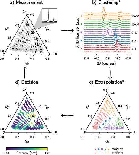
- X‑ray diffraction (XRD) patterns When X‑rays hit a crystal, they scatter and create a pattern. That pattern is like a fingerprint for the material’s structure (which crystal phase it has). The team used XRD patterns from 237 spots on a thin film containing different mixes of Fe, Ga, and Pd. For testing, they focused on 20 patterns from 5 different phase regions (4 per region), where human experts had already labeled the crystal phases. The goal: can a computer learn to label new patterns correctly with only a few examples?
- Kernels: “similarity scores” A kernel is a function that says how alike two things are. The paper compares:
- Classical kernels (run on ordinary computers):
- Radial Basis Function (RBF): measures similarity using distance between two data points (after normalizing).
- Cosine similarity: measures how well the overall shapes line up (ignores absolute size).
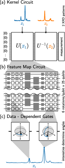
- A quantum kernel (run on a quantum computer): This uses a quantum circuit (a sequence of operations on qubits) to turn an XRD pattern into a quantum state. To compare two patterns, it runs the circuit forward for one pattern and backward for the other and asks, “Did we end up back at the starting quantum state?” If yes, they’re similar; if not, they’re different. Repeating this many times gives a similarity score.
How they tested performance:
- They trained a simple, uncertainty-aware model called a Gaussian Process classifier (think: a “smart guessing map” that also tells how sure it is) using each kernel.
- They varied how many labeled examples they gave the model (like 5, 10, 15, … out of 20) and checked how accurately it labeled the rest.
- They also used recent math tools (from other researchers) that predict when quantum kernels might have an edge, based on:
- Model complexity: roughly, how hard the model is to fit. Simpler models need less data.
- Geometric difference: a math score that tells if a classical kernel can easily imitate a quantum kernel. A large value hints that quantum might help in low-data settings.
They ran the quantum kernel both on a real trapped‑ion quantum computer (IonQ Aria) and on a noisy simulator to see the effect of hardware noise.
What they found (and why it matters)
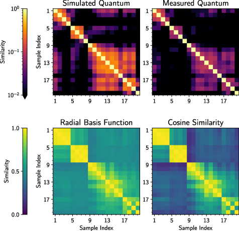
- The quantum kernel noticed subtle similarities that classical kernels missed, especially between XRD patterns with generally low peak intensities. Why? The two classical kernels they used ignore overall signal magnitude (they normalize the data), while the quantum kernel retained that information. This sometimes helped the quantum method see relationships classical methods didn’t.
- In head‑to‑head accuracy tests:
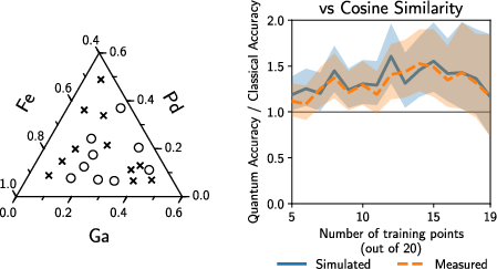
- The quantum kernel beat the RBF kernel when there were about 10 to 15 training examples. With fewer than ~10 examples, the RBF sometimes did better; with more than ~15–19, both were similar.
- The cosine similarity kernel actually performed best overall on this specific dataset. That means a very simple classical method matched the problem’s structure especially well.
- The math tests agreed with the experiments:
- The quantum kernel had lower “model complexity” than the classical ones on this dataset, which suggests it should need fewer examples to perform well.
- The “geometric difference” was large, indicating there are cases where quantum kernels can do better than classical ones in low‑data situations.
- Hardware noise mattered a bit:
- Results from the real quantum computer were close to the simulator, but slightly worse due to noise. As hardware improves, this gap should shrink.
Big takeaway: Quantum kernels can outperform some classical kernels in the small‑data regime—but not always. The best method depends on how well its assumptions match the real problem. There is no one‑size‑fits‑all winner.
What this could mean for the future
- Faster materials discovery with fewer experiments: If a quantum kernel matches the structure of a problem, it can help autonomous labs make smarter choices sooner, saving time and resources.
- Designing better quantum kernels: The paper shows that the “fit” between a kernel and the data is crucial. Future work could build quantum kernels that encode what we know about XRD patterns (for example, how peak positions and heights matter), so they learn even faster.
- Improved quantum hardware will help: Less noise means more accurate similarity scores and better learning.
- Where to use this next: The results suggest XRD and other diffraction or scattering data (which are central to materials science) may be promising targets for quantum machine learning, especially when labeled data are scarce.
In short, this study is a careful first step showing that quantum machine learning can sometimes learn complex scientific patterns with fewer examples. With smarter quantum designs and better hardware, this approach could speed up the hunt for new materials that power future technologies.
Knowledge Gaps
Knowledge gaps, limitations, and open questions
Below is a single, focused list of concrete gaps and open questions that remain unresolved by the paper and can guide future work:
- End-to-end validation in autonomy: The quantum kernel was not evaluated within a full closed-loop autonomous workflow (clustering → extrapolation → acquisition); no evidence yet that it reduces the number of XRD measurements needed to reach a target uncertainty threshold.
- Dataset scope and size: Results rely on a single ternary library with only 20 labeled XRD patterns; generalization to other materials systems, larger libraries, and real-world variability remains untested.
- Baseline strength and fairness: Only two classical baselines (RBF, cosine) with fixed hyperparameters were used; comparisons to stronger and task-specific classical baselines (e.g., dynamic time warping, earth mover’s distance, peak-shift-invariant kernels, multiple-kernel learning, SVMs, physics-informed features, or deep encoders) and with tuned hyperparameters are missing.
- Magnitude dependence vs normalization: Claimed quantum advantage may stem from using magnitude-dependent quantum encoding versus magnitude-invariant classical baselines; need to test classical magnitude-aware kernels (e.g., RBF on unnormalized intensities, weighted correlations, intensity-ratio features) and standard XRD preprocessing (thickness/orientation normalization) to isolate genuine advantages.
- Feature-map design: Only one generic, hardware-efficient feature map was tested; no systematic exploration of circuits tailored to XRD physics (e.g., shift/strain robustness, peak-width encoding, crystallographic constraints) or symmetry-inspired designs (quantum convolutional or equivariant circuits).
- Hyperparameter sensitivity (quantum): No ablation on number of qubits, number of data re-uploading layers, entangling topology, parameter scaling to [0, π], or depth; sensitivity and robustness of performance to these choices are unknown.
- Scalability and latency: The O(N2) kernel-evaluation cost with 1,024 shots per pair is not profiled for realistic active-learning scales (N ≫ 20); runtime, cost, and feasibility on cloud QPUs for time-constrained experiments are unquantified.
- Noise and error mitigation: Hardware noise reduced kernel values and performance; no exploration of error-mitigation strategies (e.g., zero-noise extrapolation, readout mitigation, PSD projection) or their impact on accuracy and stability.
- Kernel PSD integrity: Diagonals were assumed to be 1 and off-diagonals were noisy; the paper does not verify positive semidefiniteness or report PSD corrections (e.g., eigenvalue clipping) and their effect on GP performance.
- Theoretical applicability of bounds: Huang et al.’s model-complexity bound was used with multiclass labels via a one-hot mapping; the validity, tightness, and practical correlation of these bounds with multiclass GP classification error were not established.
- Acquisition design with quantum kernels: How to compute and calibrate uncertainty/acquisition functions for active learning (e.g., entropy, BALD) using quantum-XRD kernels is not addressed.
- Preprocessing pipeline: Key XRD preprocessing choices (background subtraction, smoothing, peak picking, normalization) are not detailed or evaluated; it is unclear whether the observed trends persist under standard diffraction-processing pipelines.
- Robustness to label noise: Phase labels come from human experts; sensitivity to mislabeling or borderline/multiphase samples has not been assessed.
- Modality and complexity generalization: Applicability to other scattering modalities (electron, neutron), textured samples, severe peak overlap, and 2D detector formats remains unexplored.
- Classical physics-informed baselines: No comparison to pipelines that extract physically meaningful features (e.g., peak positions/widths/intensity ratios, Rietveld-derived parameters) feeding classical learners; such baselines could invalidate perceived quantum benefits.
- Resource reporting: The paper omits time-per-kernel-element, total runtime, and cost on IonQ hardware; practical deployment requires quantitative profiling and comparison to classical compute costs.
- Statistical power and effect size: The observed advantage over RBF occurs in a narrow training-size window with very small N; broader cross-validation with larger datasets is needed to quantify effect sizes and confidence.
- Geometric difference assessment: g_CQ was computed only relative to the two chosen classical kernels; it does not rule out a well-chosen classical kernel with small g_CQ; need to optimize classical kernels first and then re-evaluate g_CQ.
- Integration with composition kernels: The system-level benefit of using a quantum kernel for XRD clustering combined with a (classical) composition kernel for extrapolation is not quantified end-to-end.
- Trainable quantum metrics: The proposal to use metric learning for feature-map discovery is not implemented; feasibility, overfitting risks in few-shot regimes, and necessary regularization remain open.
- Shift/strain invariance: Handling composition-induced peak shifts (e.g., via quantum convolution, positional encodings, or elastic alignment) is not addressed; comparison to classical shift-invariant methods (e.g., dynamic time warping) is needed.
- Shot allocation strategy: No analysis of how many shots are needed per kernel entry to achieve stable performance; adaptive shot allocation based on variance could reduce measurement cost—this is unexplored.
- Diagonal measurement: Diagonal entries k(x, x) were not measured; the impact of assuming perfect diagonals under real hardware noise on PSD and downstream GP stability is unknown.
- Transferability: Whether a learned or engineered quantum kernel generalizes across alloys/libraries (few-shot transfer) is unknown; the paper does not test cross-dataset transfer.
- Uncertainty calibration: Calibration of GP classification probabilities (e.g., reliability diagrams, Brier scores) with quantum kernels is not reported; poor calibration would harm active-learning acquisition.
- Alternative learners: Only GP classification was evaluated; whether SVMs, kernel ridge, or Nyström-approximate methods change relative performance is unknown.
- Class-wise behavior: The five-way classification performance was reported only in aggregate; which phases benefit (or suffer) with the quantum kernel, and why, is not analyzed.
- Feature resolution limits: Only 150 2θ bins were used; the impact of higher resolution, broader 2θ coverage, or multi-peak regions on qubit requirements and performance is not evaluated.
- Physics-to-circuit mapping: The conjectured link between diffraction physics (Fourier transforms, linear algebra) and quantum feature maps is not formalized; constructing kernels explicitly derived from structure-factor physics remains an open design path.
- Real-time orchestration: Practical issues for integrating a cloud QPU into an autonomous lab (batching, queue delays, fallback to classical, acquisition scheduling) are not addressed.
Glossary
- 2θ (two-theta): The diffraction angle used in XRD, representing twice the Bragg angle and serving as the horizontal axis for diffraction patterns. Example: "which captures data for a fixed range of 2 and at once."
- Active learning: A machine learning strategy that iteratively selects the most informative data points to label or measure to maximize learning efficiency. Example: "Autonomous materials science, where active learning is used to navigate large compositional phase space, has emerged as a powerful vehicle to rapidly explore new materials."
- Autonomous materials science: An automated, closed-loop approach to materials discovery that integrates experiments, modeling, and decision-making. Example: "Autonomous materials science, where active learning is used to navigate large compositional phase space, has emerged as a powerful vehicle to rapidly explore new materials."
- Bayesian surrogate model: A probabilistic model (often a Gaussian process) that approximates an expensive-to-evaluate function and quantifies uncertainty for decision-making. Example: "Autonomous experimental methods can self-navigate multi-dimensional parameter space through continuous updating of a Bayesian surrogate model without having to survey every point in the parameter space."
- Bloch sphere: A geometric representation of a single qubit’s state as a point on the unit sphere. Example: "Each group of three rotations (around the , , and axes again respectively), can describe an arbitrary rotation of the qubit Bloch sphere."
- Body centered cubic (BCC): A crystal structure with one atom at each cube corner and one atom at the cube center. Example: "Groups 1--4 and 5--8 both correspond to a body centered cubic Fe phase, but with significant peak shifting due to composition-dependent crystal lattice parameter changes \cite{long_rapid_2009}."
- Combinatorial libraries: Samples with systematically varied compositions arranged on a single substrate to enable high-throughput screening. Example: "Combinatorial libraries, where large compositional variations are laid out on individual wafers/chips, are particularly useful physical platforms for materials optimization."
- Composition spread library: A substrate containing a continuous gradient of compositions for rapid exploration of phase behavior. Example: "Specifically, we compute a quantum kernel and several classical kernels for x-ray diffraction patterns taken from an Fe-Ga-Pd ternary composition spread library."
- Conjugate transpose: For a unitary circuit, the inverse operation obtained by transposing and complex-conjugating the matrix; used to “uncompute” a feature map. Example: "applies the conjugate transpose (i.e, the inverse, because the evolution of a closed quantum system is a unitary transformation\cite{nielsen_quantum_2010}) of the feature map circuit with the data point ,"
- Cosine similarity: A similarity measure of the angle between two vectors, often used to compare patterns independent of magnitude. Example: "The cosine similarity is a simpler similarity measure which works well for clustering XRD patterns using other machine learning methods compared to more sophisticated kernels such as dynamic time warping or earth mover's distance\cite{iwasaki_comparison_2017}, but is atypical as a Gaussian process kernel because of its simplicity."
- Dynamic time warping: A distance measure for sequences that aligns them nonlinearly in time to compare shapes with temporal variations. Example: "The cosine similarity is a simpler similarity measure which works well for clustering XRD patterns using other machine learning methods compared to more sophisticated kernels such as dynamic time warping or earth mover's distance\cite{iwasaki_comparison_2017},"
- Earth mover's distance: A measure of distance between probability distributions (or histograms) interpreted as minimal “work” to transform one into the other. Example: "The cosine similarity is a simpler similarity measure which works well for clustering XRD patterns using other machine learning methods compared to more sophisticated kernels such as dynamic time warping or earth mover's distance\cite{iwasaki_comparison_2017},"
- Entropy (uncertainty): An information-theoretic measure used here to select the next experiment by maximizing uncertainty reduction. Example: "the composition with the maximum uncertainty (entropy) in its predicted label is chosen as the next composition to measure, indicated by the star."
- Feature map quantum circuit: A parameterized quantum circuit that embeds classical data into a quantum state to define a kernel. Example: "we use a feature map quantum circuit, , which receives the values of a data point ( is the number of data dimensions) as parameters and calculate..."
- Few-Shot Learning (FSL): Learning paradigms designed for regimes with very limited labeled data. Example: "The machine learning subfield of Few-Shot Learning (FSL) studies methods for such data-limited regimes \cite{parnami_learning_2022}."
- Fourier transform: A transformation between real and reciprocal (frequency) domains; central to diffraction analysis. Example: "Diffraction data might provide a data platform on which quantum kernel models can learn faster than classical kernel models because the techniques used to represent diffraction (matrix inversion and the Fourier transform) are thought to be faster on quantum computers."
- Gaussian process: A nonparametric probabilistic model over functions fully specified by a mean and covariance (kernel) function. Example: "Gaussian processes are a kernel machine learning method commonly used for the extrapolation step of the autonomous materials science workflow."
- Gaussian process classification: A GP-based probabilistic classification framework that uses kernels to model class decision boundaries with uncertainty. Example: "We used Gaussian process classification as implemented in GPflow \cite{matthews_gpflow_2017}."
- Geometric difference: A measure comparing classical and quantum kernels that upper-bounds classical model complexity relative to quantum. Example: "The geometric difference between the classical and quantum kernel, , is defined as..."
- GADDS (D8 GADDS): Bruker’s detector/software system for XRD data collection and integration. Example: "The raw detector images are then integrated to obtain the 2 angles and peak intensities using the D8 GADDS program and a script to automate the process."
- Hadamard gate: A single-qubit quantum gate creating superposition by mapping basis states to equal superpositions. Example: "The gray, 1-qubit gate is a Hadamard gate, the gray 2-qubit gate is a $\sqrt{i\text{SWAP}$ gate, and the triplets of white gates are rotation gates about the , , and axes respectively."
- Harrow Hassidim Lloyd (HHL) algorithm: A quantum algorithm for solving linear systems that can provide exponential speedups under certain conditions. Example: "which is an application where quantum computers have an exponential advantage using the Harrow Hassidim Lloyd (HHL) algorithm \cite{harrow_quantum_2009}."
- Inductive bias: The set of assumptions a learning algorithm uses to generalize beyond the training data. Example: "With this understanding, our results suggest that quantum kernel machine learning models can outperform classical kernel models, but the quantum kernel needs to have an appropriate inductive bias."
- Kernel function: A similarity function that implicitly maps data into a feature space to enable linear methods on nonlinear data. Example: "Kernel machine learning methods find patterns in data using a kernel function, , which takes two data points and as inputs and returns a value describing how similar the two data points are \cite{mengoni_kernel_2019}."
- Kernel matrix: The matrix of pairwise kernel evaluations used by kernel methods for learning and inference. Example: "This calculation is repeated for every pair of data points to construct a kernel matrix, , which is then used by the classical kernel machine learning method."
- Metric learning: Techniques that learn a task-specific similarity or distance function to improve classification or retrieval. Example: "Such a quantum kernel with appropriate inductive bias might be found using the FSL technique of metric learning."
- Model complexity (kernel-based): A quantity (per Huang et al.) that controls the upper bound on expected error given a kernel and dataset. Example: "The model complexity for kernel matrix is defined as..."
- "No Free Lunch" Theorems: Results stating no learning algorithm is universally superior across all possible problems. Example: "As highlighted by the well-known "No Free Lunch" Theorems \cite{wolpert_no_1997}, the performance of a machine learning model fundamentally depends on the specific problem it is applied to."
- One-hot encoding: A vector representation where only the component corresponding to a class label is 1 and the rest are 0. Example: "and and are the one-hot encodings of the phase labels of each composition (such that equals 1 if the labels are the same, otherwise )."
- Permutation-equivariant circuits: Quantum circuit architectures that respect symmetries under permutations, useful for structured data like graphs. Example: "such as permutation-equivariant circuits for graph learning tasks \cite{skolik_equivariant_2023} or quantum convolutional architectures for translationally symmetric data \cite{chinzei_splitting_2024}."
- Quantum advantage: A regime where a quantum method outperforms the best known classical methods on a given task. Example: "our results show that by carefully choosing a combination of problem and quantum kernel, it's possible to achieve quantum advantage for classification of x-ray diffraction patterns."
- Quantum convolutional architectures: Quantum circuit designs inspired by convolutions, exploiting translational symmetries in data. Example: "such as permutation-equivariant circuits for graph learning tasks \cite{skolik_equivariant_2023} or quantum convolutional architectures for translationally symmetric data \cite{chinzei_splitting_2024}."
- Quantum kernel: A kernel defined via inner products of quantum states prepared by a data-encoding circuit, estimated on quantum hardware. Example: "Quantum kernel machine learning is an emerging area of research that may enable certain functions to be learned with less training data than classical kernel methods, making it a promising tool for autonomous materials discovery."
- Quantum Random Access Memory (QRAM): A hypothetical quantum memory enabling superposition access to classical data indices. Example: "Quantum algorithms for accelerating kernel machine learning calculations have been developed \cite{rebentrost_quantum_2014}, but require the use of Quantum Random Access Memory \cite{mengoni_kernel_2019}, which is beyond current quantum computers."
- Radial basis function (RBF) kernel: A popular positive-definite kernel based on Gaussian similarity in Euclidean space. Example: "The squared exponential norm radial basis function kernel is a common kernel for Gaussian processes, capable of describing arbitrary functions which are sufficiently smooth \cite{rasmussen_gaussian_2008}."
- Reciprocal space: The Fourier-transformed space of periodic structures where diffraction patterns are naturally represented. Example: "The transformation from real space to reciprocal space can be written as a matrix inversion \cite{kittel_introduction_2004},"
- Singular value decomposition (SVD): A matrix factorization used to compute matrix inverses and square roots in a numerically stable way. Example: "The matrix square roots and inverses can be efficiently computed using the singular value decomposition."
- Spectral norm: The largest singular value of a matrix; used to quantify the geometric difference between kernels. Example: "... and is the spectral norm \cite{huang_power_2021}."
- √iSWAP gate: A two-qubit entangling gate equivalent to the square root of the iSWAP operation. Example: "the gray 2-qubit gate is a $\sqrt{i\text{SWAP}$ gate,"
- Stoichiometric composition: Exact atomic fractions of elements in a compound that sum to unity. Example: "The dataset consists of stoichiometric composition information, i.e. , , and in Fe\textsubscript{a}Ga\textsubscript{b}Pd\textsubscript{c} (where ),"
- Subset accuracy: The proportion of exactly correct predictions across all labels/instances in a test set configuration. Example: "To evaluate the performance of the kernels, we measured the subset accuracy of the Gaussian process classifier as a function of the number of training data points."
- Ternary phase diagram: A triangular diagram representing phase stability across three-component compositions. Example: "Autonomous optimization within libraries can be used to quickly chart materials within fixed composition variations such as ternary phase diagrams \cite{green_applications_2013}."
- Trapped ion quantum computer: A quantum processor where qubits are realized by trapped ions manipulated by lasers. Example: "we used the IonQ Aria trapped ion quantum computer for the quantum circuit execution."
- Unitary transformation: A norm-preserving linear operation in quantum mechanics representing reversible evolution. Example: "because the evolution of a closed quantum system is a unitary transformation\cite{nielsen_quantum_2010}"
- X-ray diffraction (XRD): A technique that probes crystal structure by measuring diffraction intensities as a function of angle. Example: "we evaluate how well a quantum kernel model can learn an x-ray diffraction (XRD) dataset using IonQ's Aria trapped ion quantum computer (see NIST Disclaimer)."
- ω-scan mode: An XRD measurement mode where the sample is rocked about the ω axis to record diffracted intensities. Example: "XRD of the films was performed using the -scan mode of a D8 DISCOVER for combinatorial screening (Bruker-AXS) using an x-ray beam spot size of 1 mm diameter."
Practical Applications
Immediate Applications
Below is a focused list of actionable use cases that can be deployed now, drawing directly from the paper’s methods, findings, and workflow.
- Quantum–classical hybrid XRD clustering and phase mapping in combinatorial materials libraries
- Sector: materials, manufacturing, energy, semiconductors
- Tools/products/workflows: GPflow-based Gaussian Process Classification with a quantum kernel evaluated via IonQ (or noisy simulator); autonomous “measure–cluster–extrapolate–decide” loop for ternary/ternary-like phase mapping
- Dependencies/assumptions: access to cloud QPU or high-fidelity simulator; manageable device noise; small-to-moderate dataset sizes (tens to low hundreds of patterns); intensity-preserving preprocessing (scaling to [0, π]); fixed hyperparameters sufficing for early-stage exploration
- Active learning prioritization for autonomous labs (fewer XRD measurements to reach a target uncertainty)
- Sector: robotics/lab automation, materials informatics
- Tools/products/workflows: a scheduling plugin that uses quantum-kernel-based uncertainty/entropy to pick the next composition; integration with combinatorial XRD systems (e.g., Bruker D8) and lab orchestration software
- Dependencies/assumptions: tight instrument–software integration; reliable kernel evaluations (≥1,024 shots per pair); cost-aware selection (O(N²) kernel pairs)
- Retrospective analysis of archival XRD to reveal low-intensity phase relationships missed by magnitude-invariant measures
- Sector: materials characterization, data curation
- Tools/products/workflows: “Quantum Kernel Audit” service for existing diffraction repositories; on-demand cloud microservice to compute kernel matrices highlighting faint similarities
- Dependencies/assumptions: availability of raw (non-normalized) intensity traces; compute budgets for pairwise kernel calls; acceptance of hardware-noise-induced variability
- Task triage via Huang et al.’s model complexity and geometric difference metrics (choose quantum vs. classical per task)
- Sector: R&D portfolio management (academia/industry), materials informatics
- Tools/products/workflows: lightweight Python package that computes s_K and g_CQ to decide when a quantum kernel is likely helpful in data-limited regimes
- Dependencies/assumptions: ability to invert/square-root kernel matrices; representative pilot datasets; team familiarity with kernel diagnostics
- Immediate curriculum and training modules using the open GitHub repository
- Sector: education, workforce development
- Tools/products/workflows: hands-on lab assignments replicating the Fe–Ga–Pd results; exercises comparing cosine/RBF vs. quantum kernels; exposure to GPflow, IonQ API, and Few-Shot Learning concepts
- Dependencies/assumptions: student access to simulator (or limited QPU credits); reproducible environments; instructor familiarity with Gaussian processes and basic quantum circuits
- LIMS and laboratory software integration of quantum-kernel evaluation as a microservice
- Sector: lab software vendors, contract research organizations
- Tools/products/workflows: REST API to request kernel matrices for XRD batches; plug-ins for phase mapping dashboards
- Dependencies/assumptions: secure cloud integrations; SLA considerations for QPU jobs; data governance and audit trails (esp. with third-party clouds)
- Rapid pilot extensions to electron or neutron diffraction datasets (same vector-intensity paradigm)
- Sector: structural characterization across modalities
- Tools/products/workflows: swap the input vectors and scaling; reuse the same Peters-style feature map circuit for magnitude-sensitive kernels
- Dependencies/assumptions: proper intensity normalization; validation on small pilot datasets; awareness of domain-specific artifacts (e.g., background subtraction)
- Evidence-based funding and program decisions (policy-facing whitepapers)
- Sector: policy/funders (agencies, foundations), research administration
- Tools/products/workflows: briefings that justify quantum kernel allocation when geometric difference is large and training data are limited
- Dependencies/assumptions: transparent reporting of costs and accuracy gains; standardized benchmarking results to persuade reviewers
Long-Term Applications
These use cases require further research, scaling, hardware advances, or tailored feature-map design to realize their full potential.
- Fully autonomous materials discovery pipelines with task-specific quantum feature maps and robust quantum advantage
- Sector: energy storage, catalysis, semiconductors, magnetic materials
- Tools/products/workflows: “QKernel-AL” platform integrating custom feature maps for diffraction; closed-loop optimization across synthesis and characterization
- Dependencies/assumptions: improved QPU fidelity and scale; metric learning to tailor feature maps to diffraction physics; standardized uncertainty targets and success metrics
- Accelerated discovery of high-impact materials (battery electrodes, solid electrolytes, catalysts, superconductors, wear-resistant alloys)
- Sector: energy, transportation, electronics, industrial manufacturing
- Tools/products/workflows: high-throughput combinatorial libraries guided by quantum kernels; multi-objective optimization (performance, stability, cost)
- Dependencies/assumptions: large-scale high-throughput infrastructure; robust handling of multi-modal data (XRD + composition + property assays); sustained cost-effectiveness vs. classical baselines
- Standardized quantum-kernel benchmarking suite for diffraction data and data-limited regimes
- Sector: academia/industry consortia, standards bodies
- Tools/products/workflows: open datasets, leaderboards, and metric implementations (model complexity, geometric difference, accuracy vs. shot count)
- Dependencies/assumptions: community consensus on tasks and metrics; sponsorship by national labs or standards organizations; reproducibility across QPU vendors
- Cross-modal kernel fusion (composition kernels + quantum XRD kernels) for more reliable active learning decisions
- Sector: materials informatics, autonomous labs
- Tools/products/workflows: multi-kernel Gaussian processes; uncertainty-aware experiment planning across composition and structural signals
- Dependencies/assumptions: principled kernel combination strategies; careful calibration of uncertainties; systematic validation against expert labels
- Quantum metric learning and automated feature-map search for diffraction
- Sector: software/AI tooling, quantum ML
- Tools/products/workflows: AutoML-style pipeline that learns quantum circuit ansätze matching problem inductive biases; generalization to related domains (peak-shift tolerance, background handling)
- Dependencies/assumptions: availability of training signal without prohibitive QPU cost; efficient gradient-free/gradient-based search in noisy settings; transferability across datasets
- Real-time, on-instrument inference (near-edge QPU or accelerated simulators for high-throughput XRD)
- Sector: industrial R&D, fabs, pilot plants
- Tools/products/workflows: low-latency kernel evaluation for immediate phase assignment and adaptive sampling during scans
- Dependencies/assumptions: edge/QPU hardware availability; reliable connectivity; strong error mitigation to support continuous operations
- Extension to Fourier-transform-heavy domains beyond materials (where magnitude and phase carry diagnostic value)
- Sector: healthcare (medical imaging QA, certain spectroscopy), geophysics/seismology, nondestructive testing
- Tools/products/workflows: quantum-kernel-based classifiers for spectral patterns; anomaly detection in low-signal environments
- Dependencies/assumptions: domain adaptation; regulatory and validation requirements (e.g., medical device approval); robust pipelines for clinical/field deployment
- Enterprise-grade microservices: “Quantum-accelerated Phase Mapping” as a product offering
- Sector: materials informatics vendors, contract labs
- Tools/products/workflows: subscription service providing kernel computation, phase map extrapolation, and experiment scheduling support
- Dependencies/assumptions: cost model favorable vs. classical compute; QPU uptime and vendor lock-in considerations; customer data privacy and compliance
- National strategy and infrastructure for quantum-enabled autonomous labs
- Sector: policy/government, national labs
- Tools/products/workflows: coordinated investment in QPU access, training programs, and standardized interfaces (LIMS, robotic platforms)
- Dependencies/assumptions: convincing evidence of advantage in prioritized domains; workforce development; inter-agency collaboration
- Downstream daily life impacts: faster deployment of improved consumer products (longer-lasting batteries, lighter alloys, efficient catalysts)
- Sector: consumer electronics, automotive, appliances
- Tools/products/workflows: accelerated R&D pipelines feeding product lines; sustainability gains via reduced experimental waste
- Dependencies/assumptions: end-to-end integration from discovery to scale-up; manufacturing readiness; regulatory and safety validation
Notes on overarching assumptions and dependencies:
- Quantum hardware: fidelity, qubit count, noise, and shot budgets significantly affect kernel estimates and reliability.
- Data regime: advantages are most likely in data-limited settings; as datasets grow large, classical models may catch up or surpass unless feature maps encode superior inductive bias.
- Preprocessing: magnitude-preserving transformations are crucial when leveraging the quantum kernel’s sensitivity to intensity.
- Cost and latency: pairwise kernel evaluation scales quadratically, requiring careful batching, caching, or subsampling.
- Generalization: results demonstrated on Fe–Ga–Pd XRD; broader adoption needs validation across compositions, modalities, and tasks.
- Standards and reproducibility: shared benchmarks and open code/data (as in the paper’s GitHub) will be key to adoption.
Collections
Sign up for free to add this paper to one or more collections.