Modeling Cosmogenic 10Be During the Heliosphere's Encounter with an Interstellar Cold Cloud
Abstract: Geologic records of cosmogenic 10Be are sensitive to changes in the radiation environment with time. Recent works suggest there are periods when the Sun encountered massive cold clouds which compressed the heliosphere to within Earth's orbit. This would expose Earth to increased galactic cosmic rays and MeV-energy particles of heliospheric origin. We model 10Be production in Earth's atmosphere during possible cold cloud encounters, and estimate their detectability in marine records of variable temporal resolution. We find that an AU-scale cold cloud encounter can be detected using ocean sediment measurements of 10Be if Earth spends time inside the compressed heliosphere. For typical relative speeds between the Sun and local interstellar clouds, this translates to a crossing time of ~100 years. A cloud must have an extension on the scale of parsecs to tens-of-parsecs (crossing time 0.1-1 Myr) to be detectable through 10Be measurements in iron-manganese crusts.
Paper Prompts
Sign up for free to create and run prompts on this paper using GPT-5.
Top Community Prompts
Explain it Like I'm 14
What this paper is about (big picture)
Imagine the Sun surrounds us with a protective bubble made by the solar wind—this bubble is called the heliosphere. Sometimes, as the Sun travels through the galaxy, it may run into dense, very cold clouds of gas. These clouds squeeze the heliosphere smaller. When that happens, more high‑energy particles from space can reach Earth.
This paper asks: if the heliosphere got squeezed by one of these clouds in the past, would Earth’s atmosphere make extra amounts of a special atom called beryllium‑10 (written as 10Be), and could we spot that spike today in ocean rocks and sediments?
The main questions in simple terms
The authors set out to answer:
- How much extra 10Be would Earth make during a “cloud squeeze” event?
- Would that extra 10Be show up clearly in ocean sediments or in very slow‑growing seafloor crusts?
- How big and how long would a cloud crossing need to be for us to notice it in those records?
How they studied it (methods made simple)
Think of cosmic rays like invisible “space rain” made of fast particles. When these particles hit the air, they trigger chain reactions that create 10Be in the atmosphere. That 10Be eventually falls into the ocean and gets locked into sediments and metal crusts on the seafloor, where scientists can measure it millions of years later.
To estimate how much 10Be gets made, the team used:
- A computer model (CRAC) that simulates how incoming particles make 10Be in the atmosphere.
- Different “space weather” scenarios:
- Normal conditions inside today’s heliosphere (our usual protective bubble).
- Earth outside the bubble, exposed to pure galactic cosmic rays (GCRs) from the wider galaxy.
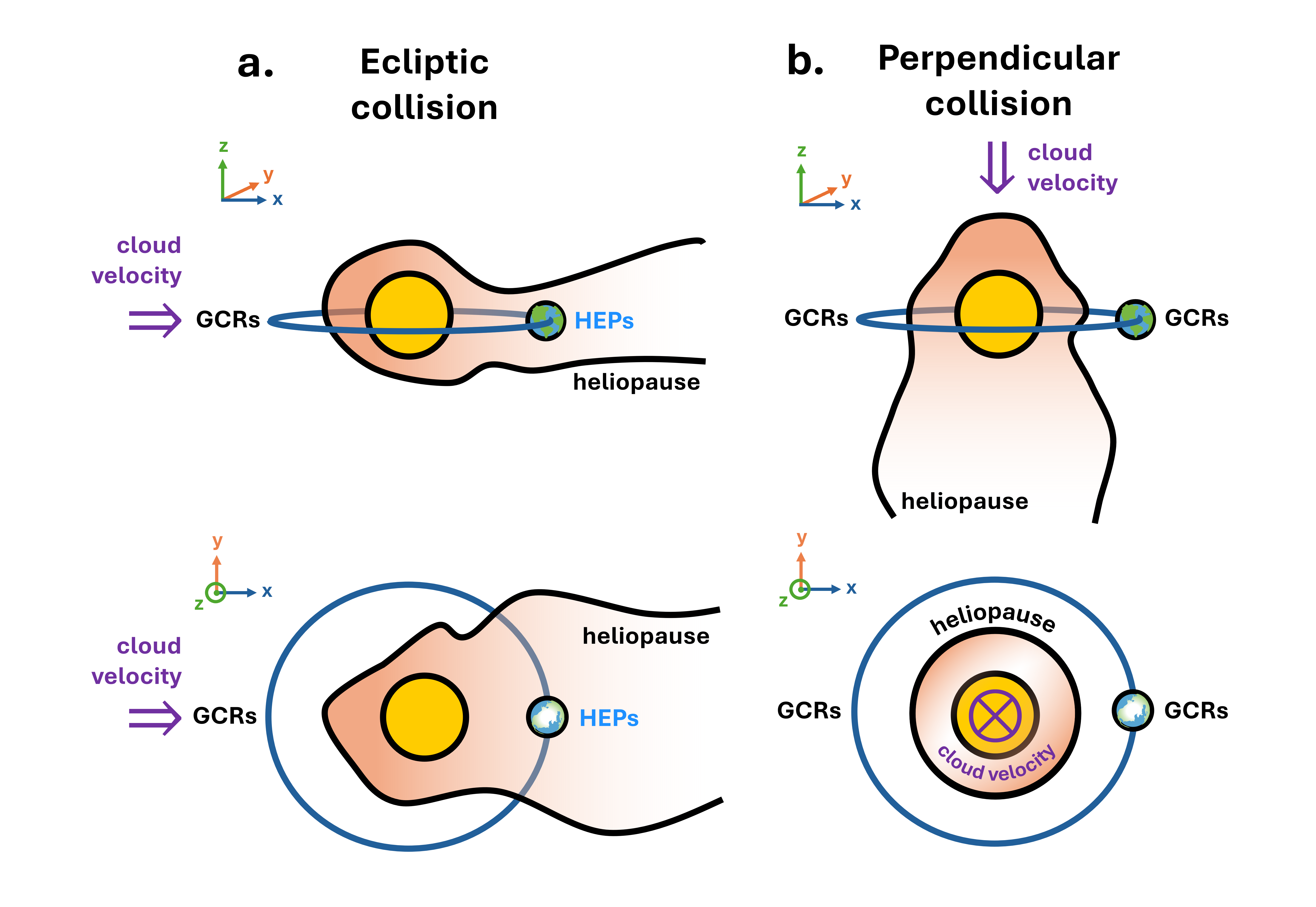
- Earth dipping back into a strongly compressed heliosphere with lots of heliospheric energetic particles (HEPs)—these are particles energized by shocks in the squeezed bubble.
They also tested different cloud sizes and crossing times:
- Short: about 100 years (hundreds of times the Earth‑Sun distance, called AU).
- Medium: about 100,000 years (0.1 million years, or roughly 2 parsecs).
- Long: about 1 million years (around 20 parsecs; 1 parsec ≈ 3.26 light years).
Finally, they asked if the extra 10Be would stand out clearly in:
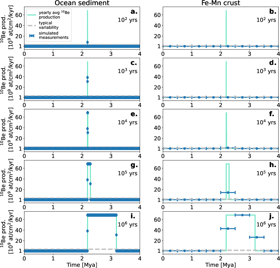
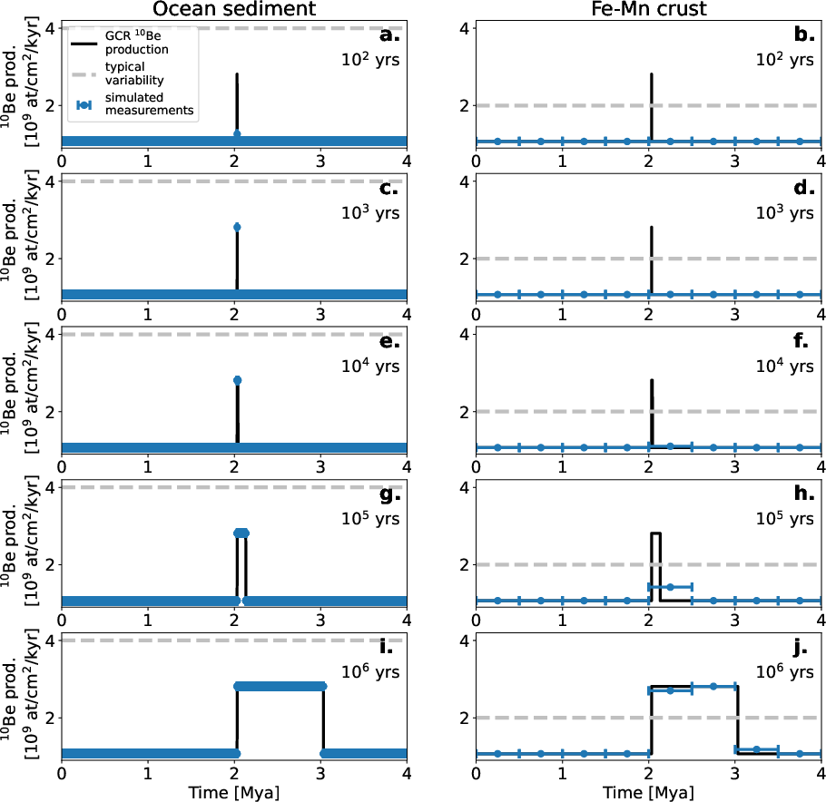
- Ocean sediments (fine layers that average about 1,000 years per sample—high time resolution).
- Iron‑manganese crusts (very slow‑growing layers that average about 200,000–1,000,000 years per sample—low time resolution).
What they found and why it matters
Here are the key takeaways:
- If Earth gets exposed to heliospheric energetic particles (HEPs) during a compressed‑bubble event, 10Be production skyrockets. Globally, it can jump roughly 270 times above normal; near the poles, even more. That’s a huge, obvious signal.
- If Earth is only exposed to galactic cosmic rays (GCRs) without the HEPs, 10Be increases by less than about 3 times—this is small and can be masked by natural Earth changes (like climate and circulation), making it harder to spot.
- Detectability depends on how long the crossing lasts and which particles reach Earth:
- Short crossings (~100 years; AU‑scale clouds): Likely detectable in ocean sediments only if HEPs reach Earth (for example, if Earth dips in and out of the compressed heliosphere during its orbit). Not detectable in iron‑manganese crusts.
- Medium crossings (~0.1 million years; ~2 parsecs): Clear in ocean sediments with many samples across the peak; might be very limited or even invisible in iron‑manganese crusts if only GCRs are involved.
- Long crossings (~1 million years; ~20 parsecs): Detectable in both sediments and crusts; even GCR‑only cases may be seen, though they’re less distinct and can be confused with other Earth causes.
- Real data fits this picture: One study found a 10Be increase about 9–11 million years ago lasting 1–2 million years (a small, long hump). That looks like the GCR‑only case—consistent with a long, gentle crossing and little or no HEP exposure. Meanwhile, other proposed crossings around 2–3 or 6–7 million years ago haven’t shown up in low‑resolution records, suggesting those events—if they happened—were short (too brief for iron‑manganese crusts to resolve).
In short:
- HEP exposure creates a big, obvious 10Be spike.
- GCR‑only exposure makes a modest, harder‑to‑see bump.
- Ocean sediments can reveal short events; iron‑manganese crusts mostly catch long ones.
Why this research is important (implications)
- It gives scientists a “rulebook” for spotting past space‑environment changes in Earth’s rocks. Knowing when the heliosphere was squeezed helps us understand how the Solar System interacted with its galactic neighborhood.
- It tells us which archives to use: look to ocean sediments for short, sharp events; use iron‑manganese crusts for long, gentle ones.
- It helps test big ideas about our past: If we find the predicted 10Be spikes, that supports the theory that the Sun crossed dense cold clouds that compressed the heliosphere.
- More broadly, it connects astrophysics and Earth science—showing how the galaxy’s environment can leave fingerprints in our planet’s geological record.
A few helpful translations of terms
- Heliosphere: The Sun’s protective bubble made by the solar wind.
- AU (astronomical unit): The distance from Earth to the Sun (~150 million km).
- Parsecs (pc): A big space distance; 1 pc ≈ 3.26 light years.
- GCRs (galactic cosmic rays): High‑energy particles from across the galaxy.
- HEPs (heliospheric energetic particles): Particles boosted in energy by shocks at the edge of a strongly compressed heliosphere.
- 10Be (beryllium‑10): A rare, long‑lived atom made in the atmosphere by cosmic rays; it settles into ocean sediments and seafloor crusts, acting like a time‑stamped “breadcrumb” of past radiation.
Knowledge Gaps
Knowledge gaps, limitations, and open questions
The following bullet list enumerates specific knowledge gaps, limitations, and open questions left unresolved by the paper that future work could address:
- Cloud properties are poorly constrained: actual sizes, column densities, temperatures, ionization fractions, magnetic fields, and geometries (sheet/filament vs. clumpy) of candidate cold clouds near the Sun remain unknown, making crossing durations and heliospheric compression uncertain.
- Directionality of encounters is not constrained: the relative orientation of cloud motion to the ecliptic and the heliotail shape determine Earth’s HEP/GCR exposure fraction; no 3D, time-dependent heliosphere–cloud interaction model is used to quantify realistic exposure ratios beyond the assumed 80% GCR/20% HEP case.
- HEP spectrum uncertainties: the HEP spectrum is taken from a single model and spline-extrapolated to higher energies; there is no validation against observations or physics-based acceleration limits for a parallel termination shock under cold-cloud conditions.
- Energy-dependent production uncertainty: 10Be yield at MeV energies (where HEPs dominate) is sensitive to cross-section thresholds and GEANT4 physics lists; the paper does not quantify how uncertainties in low-energy spallation yields propagate to the 70× production enhancement claim.
- Particle composition gaps: production modeling only includes primary protons and α-particles; contributions from heavier nuclei (in both GCRs and HEPs) are not assessed and could alter 10Be yields and latitudinal deposition patterns.
- HEP angular distribution and temporal variability: potential anisotropy and time variability of HEPs (seasonal, orbital-phase dependent, shock geometry changes) during a compressed-heliosphere crossing are not characterized.
- Cloud-induced GCR attenuation is simplified: attenuation is assumed negligible aside from a cited ~10% reduction at 100 MeV; effects across the full GCR spectrum, and additional attenuation by cloud magnetic turbulence or dust, are not modeled.
- Solar wind and shock physics in dense clouds: how cold-cloud ram, thermal, magnetic, and ionization pressures reshape heliospheric shocks (strength, geometry, turbulence, acceleration efficiency) and hence the HEP spectrum and flux is not explored.
- Geomagnetic field treatment is static: the model holds the dipole moment constant at present-day values; realistic Pliocene–Pleistocene dipole intensity variations, reversals/excursions, tilt, and secular variation are not incorporated and could materially change production and latitudinal deposition.
- Atmospheric transport is neglected: no coupling to stratosphere–troposphere exchange, meridional transport, and precipitation; therefore, polar production may overestimate deposition by 20–50%, and site-specific deposition patterns remain unquantified.
- Oceanic and sedimentary confounders: variability in sedimentation rates, bioturbation, diagenesis, lateral transport, and basin-specific scavenging of Be are not modeled; their impact on detectability thresholds and signal distortion is not quantified.
- 10Be/9Be ratio modeling is absent: the analysis references that both flux and 10Be/9Be are used in practice, but does not simulate or assess how variable 9Be supply and scavenging could help isolate production changes from depositional/climatic noise.
- Fe–Mn crust growth-rate variability: smoothing and variable growth rates (mm/Myr) and microstratigraphic heterogeneities in crusts are not incorporated, yet they directly affect detectability and apparent peak duration; no sensitivity analysis is provided.
- Statistical detection framework is missing: detectability is judged against “typical variability” (2–4× in sediments, 1–2× in crusts) without a formal signal-to-noise model, Monte Carlo uncertainty propagation, or Bayesian detection criteria tied to real datasets.
- Site selection and spatial heterogeneity: results are presented as global/polar averages; actionable guidance on optimal core locations (latitude, precipitation regime, ocean basin) to maximize 10Be signal-to-noise for short crossings is not developed.
- Baseline GCR variability over Myr: the paper assumes present-day-like solar/ISM modulation outside crossings; potential long-term changes in the LIS (Local Interstellar Spectrum), solar activity, or galactic environment are not explored.
- Concurrent GCR modulation inside compressed heliosphere: during the 20% “inside” phase, the model uses HEP-only exposure; modulation of GCRs inside the compressed heliosphere (which might be stronger/weaker than modern) is not explicitly included or constrained.
- Age-model uncertainties: detectability claims do not incorporate chronological errors in sediments or crusts (e.g., tuning, hiatuses), which can blur short-lived signals and complicate correlation with predicted crossing windows.
- Alternative astrophysical sources: distinguishing a cold-cloud crossing signal from supernovae, solar superflares, or geomagnetic excursions is not addressed; multi-proxy approaches to attribution are not proposed.
- Ice-core records for short events: the potential of polar ice cores (with annual–decadal resolution) to capture 100–1000-year crossings with strong polar 10Be production is not evaluated against realistic post-depositional processes and dating uncertainties.
- Cross-isotope validation: coordinated modeling and measurement of other cosmogenic nuclides (e.g., 26Al, 36Cl, 14C) are not performed, limiting the ability to verify a cold-cloud crossing via isotopic co-variations and energy-dependent signatures.
- Event-shape characterization: the paper suggests that high-density sediment sampling could resolve 100 kyr peaks, but does not investigate how cloud geometry (filament vs. sheet), intermittency, or multi-pass encounters translate into characteristic peak shapes distinguishable from climate-driven variability.
- Calibration to existing records: predictions for 2–3 and 6–7 Mya crossings are not confronted with curated high-resolution 10Be sediment datasets from those intervals to empirically test detectability under realistic noise and age control.
- Uncertainty quantification is limited: no comprehensive error bars on modeled production rates (from spectra, yields, geomagnetic parameters, transport, deposition), making the confidence in the claimed 70× enhancement and detectability thresholds difficult to assess.
- Methodological reproducibility details: key inputs (exact HEP spectrum, spline parameters, rigidity cutoff implementation, yield-function selections) and their sensitivity ranges are not fully specified for independent replication and stress testing.
Practical Applications
Immediate Applications
- Targeted ocean-sediment sampling to test recent cold-cloud crossings
- Sectors: academia (geosciences, heliophysics), instrumentation (AMS labs), marine coring industry
- What to do: Prioritize 1 cm sampling (≈1 kyr resolution) across 2–3 Ma and 6–7 Ma intervals in high-accumulation marine sediment cores; increase sampling density to resolve 5–10 kyr-scale peaks; compute both 10Be flux and 10Be/9Be ratios; co-analyze with paleointensity records to separate geomagnetic vs heliospheric effects.
- Tools/workflows: Use CRAC-based planning calculators to predict Be-10 detectability vs sampling resolution; adopt standardized reporting of sedimentation rates and time integration per aliquot.
- Assumptions/dependencies: Earth must have experienced periodic HEP exposure (e.g., ≈20% of orbit) during an AU-scale crossing; accurate age models for cores; local depositional processes not masking >4× anomalies.
- Event-flagging thresholds for stratigraphers using 10Be
- Sectors: academia (stratigraphy, paleoceanography), energy (stratigraphic correlation services)
- What to do: Apply simple triage rules—HEP+GCR scenarios produce up to ~70× global 10Be increases (well above 2–4× “typical variability”), while GCR-only scenarios yield ≤3× (hard to discriminate) unless ≥0.5–1 Myr duration.
- Tools/workflows: Automated peak detection with tunable thresholds aligned to archive-specific variability; cross-check against Fe–Mn crusts (0.5 Myr resolution) for Myr-long events.
- Assumptions/dependencies: Variability bands (2–4× sediments; 1–2× crusts) hold for target sites; no large diagenetic artifacts.
- Improved correction protocols for cosmogenic 10Be applications (surface exposure dating, erosion rates)
- Sectors: academia and industry (geomorphology, geochronology consultancies), AMS labs
- What to do: Include a “heliospheric compression” term in production-rate corrections when interpreting anomalous high-10Be intervals in long records; flag time windows with suspected astrophysical boosts to avoid misattributing to climate or erosion.
- Tools/workflows: Incorporate paper-derived HEP and GCR production scenarios into production-rate calculators; propagate polar vs global deposition biases with mixing corrections (20–50% lower polar deposition than polar production).
- Assumptions/dependencies: Reliable age control; depositional continuity; use of modern-like geomagnetic dipole moment (as assumed in the model).
- Cross-archive multi-proxy study design (ocean sediments, Fe–Mn crusts, ice cores, lunar soil)
- Sectors: academia (Earth/planetary), space agencies
- What to do: Plan coordinated campaigns where short events (100–1,000 yr) are probed in high-resolution marine/ice archives and long events (0.1–1 Myr) in Fe–Mn crusts and lunar 26Al; exploit complementary sensitivity windows.
- Tools/workflows: A detectability matrix that maps event duration and particle exposure (HEP vs GCR) to archive/time-resolution pairs; repository of candidate intervals and sites.
- Assumptions/dependencies: Inter-archive synchronization; sufficient analytical precision for 26Al (if used) and 10Be.
- Sediment core site selection and sampling-density calculators
- Sectors: academia, marine operations
- What to do: Use the study’s production-rate boosts (HEP: ~270× global, ~1450× polar; GCR-only: ≤3×) to set minimum sampling density and core-quality requirements by hypothesized event duration (100 yr to 1 Myr).
- Tools/workflows: Open-source calculator that ingests accumulation rate, analytical precision, and hypothesized event geometry (ecliptic vs perpendicular) to output required sampling plans.
- Assumptions/dependencies: Local chemo-sedimentary variability within expected ranges; accurate accumulation-rate estimates.
- AMS laboratory QA/QC updates for extreme 10Be peaks
- Sectors: instrumentation (AMS vendors, labs)
- What to do: Check dynamic range, standards, and dilution protocols to handle potential 10Be spikes up to tens-of-fold above background without saturation or memory effects.
- Tools/workflows: High-activity standard sets; inter-lab round robins for high-10Be samples.
- Assumptions/dependencies: Availability of suitable standards; stable ion source performance.
- Funding and policy guidance for “short-event” detection campaigns
- Sectors: policy/funding agencies, academia
- What to do: Prioritize proposals that target high-resolution ocean sediments to test AU-scale encounters (≤100–1,000 yr) given crusts’ insufficiency at this scale; support cross-lab calibration efforts.
- Tools/workflows: Program calls referencing detectability criteria and cross-archive designs; data-sharing mandates aligned with the paper’s open-data ethos.
- Assumptions/dependencies: Sufficient core availability; ship time and lab capacity.
- Education and outreach modules on heliosphere–ISM interactions via cosmogenic records
- Sectors: education, public outreach
- What to do: Develop course labs where students use provided spectra (GCR, HEP) and yield functions to simulate 10Be signals for different cloud geometries and durations.
- Tools/workflows: Jupyter notebooks built on CRAC-style yield functions; parameter sliders for HEP/GCR ratios and geomagnetic strength.
- Assumptions/dependencies: Access to curated datasets (e.g., Nica et al. 2025 Open Research).
Long-Term Applications
- Global chronostratigraphic markers for Myr-scale encounters
- Sectors: academia (stratigraphy), energy (subsurface correlation)
- What to do: If validated, define “cold-cloud encounter horizons” as correlatable markers in Fe–Mn crusts and sediments, especially for 0.5–2 Myr events with sustained GCR-only peaks (~1.5–2×).
- Tools/workflows: A global database of candidate horizons and correlation software integrating 10Be with other isotopes and paleomagnetism.
- Assumptions/dependencies: Confirmation of one or more Myr-long events and robust age control.
- Coupled heliosphere–magnetosphere–atmosphere chemistry modeling
- Sectors: academia (space physics, atmospheric chemistry), climate research
- What to do: Build 3D models to propagate HEP/GCR inputs through geomagnetic shielding and atmospheric cascades into chemistry (NOx/ozone) and radiative impacts; assess biospheric and climate implications.
- Tools/workflows: Integrated MHD–transport models, GEANT4-based cascade modules, and chemistry–climate models.
- Assumptions/dependencies: Better constraints on HEP spectra, geomagnetic state, and cloud properties; computational resources.
- Space weather risk scenarios for heliospheric compression events
- Sectors: aerospace (satellites, aviation), policy
- What to do: Develop worst-case radiation environment scenarios for rare heliosphere–cloud encounters to inform deep-time risk registries and resilience planning.
- Tools/workflows: Radiation environment models tied to asset vulnerability (SEUs, dose, avionics); long-horizon risk frameworks.
- Assumptions/dependencies: Event probability, timing, and spectra remain highly uncertain; mainly strategic foresight rather than operational forecasting.
- Artemis and future lunar sampling strategies for 26Al and 10Be
- Sectors: space agencies, planetary science
- What to do: Design regolith sampling at depth and time-resolution sufficient to detect ≥100 kyr events; extend to in situ or return-sample measurements of 26Al and 10Be.
- Tools/workflows: Landing site selection with minimal gardening; depth profiling protocols; improved AMS and potential in situ detectors.
- Assumptions/dependencies: Mission timelines and instrumentation readiness; surface disturbance history.
- Instrument development: high-throughput, wide dynamic range cosmogenic isotope measurement
- Sectors: instrumentation industry, AMS labs
- What to do: Develop AMS upgrades and reference materials that maintain precision across background to >70× spikes; automation for dense sampling campaigns.
- Tools/workflows: New ion sources, detectors, and data pipelines; certified reference materials at multiple activity levels.
- Assumptions/dependencies: Market demand from expanded cosmogenic programs.
- Decoupling geomagnetic and heliospheric signals in paleorecords
- Sectors: academia (paleomagnetism, geochronology)
- What to do: Joint inversion frameworks that use paleointensity data plus 10Be/26Al to attribute variance to geomagnetic modulation vs heliospheric compression; refine global dipole reconstructions.
- Tools/workflows: Bayesian data assimilation pipelines combining rock-magnetic and cosmogenic datasets.
- Assumptions/dependencies: Quality and density of paleointensity records; standardized uncertainties.
- Mars and other planetary archives for interstellar encounter signatures
- Sectors: planetary science, space agencies
- What to do: Assess feasibility of detecting compressed-heliosphere-like cosmogenic anomalies in Martian regolith or icy moon surfaces as comparative tests.
- Tools/workflows: Planet-specific cascade and deposition models; mission payload studies.
- Assumptions/dependencies: Availability of high-quality samples; differences in atmospheres and magnetospheres.
- Commercial and governmental data services for cosmogenic event analytics
- Sectors: energy (subsurface correlation), environmental consultancies, agencies
- What to do: Offer curated, versioned cosmogenic isotope datasets with event annotations, detectability scores, and correlation tools for stratigraphic projects.
- Tools/workflows: SaaS platforms with APIs to query 10Be peaks and metadata; integration with core repositories.
- Assumptions/dependencies: Community buy-in and sustained data contributions.
- Standards for reporting and archiving high-resolution 10Be data
- Sectors: journals, data repositories, funding agencies
- What to do: Establish minimum metadata (accumulation rate, depth-to-time model, integration per sample, local variability) and open-access deposition for interoperability with detectability models.
- Tools/workflows: FAIR-aligned repositories; submission checklists; community schemas.
- Assumptions/dependencies: Editorial and funder enforcement; lab compliance.
- Early-warning science (very long horizon): local ISM mapping
- Sectors: astronomy, policy
- What to do: Invest in high-resolution mapping of nearby cold clouds (sizes, densities, kinematics) to bound probabilities and timing of future encounters on 104–106 yr horizons.
- Tools/workflows: UV/optical/radio surveys; data assimilation into heliosphere trajectory models.
- Assumptions/dependencies: Survey coverage and sensitivity; trajectory uncertainties over long timescales.
Notes on dependencies shared across applications:
- Geometry matters: Ecliptic-plane encounters enabling periodic HEP exposure are essential for detecting ≤0.1 Myr events in sediments; perpendicular encounters (GCR-only) generally require ≥0.5–1 Myr to register in Fe–Mn crusts.
- Atmospheric mixing not modeled here likely reduces polar deposition by ~20–50% relative to polar production; apply corrections in polar archives.
- Geomagnetic field assumed near modern values; deviations alter cutoffs and production rates.
- GCR attenuation within clouds is modest (≤10% at ~100 MeV), but high-density clouds could dampen signals.
- Analytical precision and accurate age models are critical to discriminate 2–4× background variability from astrophysical signals.
Glossary
- Aluminum-26 (Al): A cosmogenic radionuclide of aluminum used as a tracer, with a half-life suitable for million-year scale events. " has a half-life of 0.7 Myr"
- Alpha particles (α-particles): Helium nuclei used as primary particles in cosmic-ray simulations of atmospheric cascades. "for primary protons and -particles with energies 20 MeV-100 GeV."
- Astronomical unit (AU): The average Earth–Sun distance (~150 million km), used to express heliospheric and cloud scales. "Today, the heliopause extends to 120 AU in the Sun's direction of motion"
- Atmospheric mixing: Transport processes that redistribute isotopes after production, affecting deposition patterns. "We do not account for atmospheric mixing"
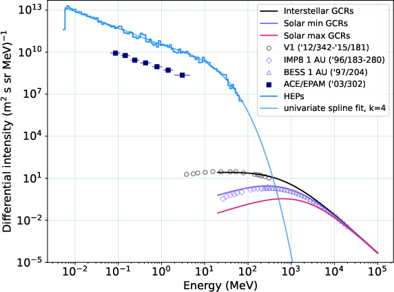
- BESS balloon flight: A balloon-borne experiment that measured cosmic-ray spectra used for comparison. "Purple points represent data from a BESS balloon flight in 1997"
- Column density: The integrated number of particles along a line of sight through a medium, affecting cosmic-ray attenuation. "within a cloud with a column density similar to the estimated size of the Local Leo Cold Cloud"
- Day of Year (DOY): A sequential count of days used to timestamp spacecraft observations. "from DOY 342 of 2012 to DOY 181 of 2015."
- Ecliptic plane: The plane of Earth’s orbit around the Sun, relevant for collision geometries with interstellar clouds. "a collision with a cold cloud in the ecliptic plane"
- Energy cutoff: The minimum particle energy required to penetrate geomagnetic shielding and contribute to production. "Integration over energy begins above the energy cutoff for each species"
- Galactic cosmic rays (GCRs): High-energy charged particles originating outside the Solar System that modulate isotope production. "The heliosphere shields Earth from interstellar galactic cosmic rays (GCRs)"
- GEANT4: A Monte Carlo simulation toolkit used to model particle interactions and yield functions. "using the GEANT4 simulation"
- Geomagnetic dipole moment: A measure of Earth’s magnetic field strength affecting cosmic-ray cutoff rigidities. "We apply a geomagnetic dipole moment Am"
- Geomagnetic equator: The region of minimal geomagnetic latitude where shielding is strongest. "near the geomagnetic equator"
- Geomagnetic shielding: Deflection of charged particles by Earth’s magnetic field, limiting low-energy penetration. "they do not penetrate geomagnetic shielding at equatorial latitudes"
- GeV: Giga–electron volts, an energy unit for high-energy particles. "70 MeV - 5 GeV"
- Halloween Storm of 2003: A major solar energetic particle event used as a reference for extreme fluxes. "Navy squares show SEP fluxes during the Halloween Storm of 2003, one of the largest recorded solar storms"
- Heliopause: The boundary where the solar wind pressure balances the ISM, defining the heliosphere’s outer edge. "Today, the heliopause extends to 120 AU"
- Heliosphere: The solar-wind–generated bubble that shields the Solar System from interstellar radiation. "The heliosphere shields Earth from interstellar galactic cosmic rays (GCRs)"
- Heliospheric energetic particles (HEPs): Particles accelerated at the compressed heliospheric termination shock during cloud encounters. "HEPs are produced when energetic particles in the solar wind are accelerated at the termination shock of the compressed heliosphere."
- IMP8: A spacecraft that measured cosmic rays near Earth, used for spectral comparison. "and from IMP8 in 1996."
- Interstellar cold cloud: Dense, cold ISM structures that can compress the heliosphere and alter radiation exposure. "suggest an interstellar cold cloud crossing as a possible explanation."
- Interstellar medium (ISM): The gas and dust between stars through which the Sun travels. "the interstellar medium (ISM)"
- keV: Kilo–electron volts, an energy unit for lower-energy particles. "accelerates high fluxes of energetic particles from keV to MeV energies"
- Local Leo Cold Cloud: A nearby cold cloud hypothesized to be a thin sheet, affecting crossing durations. "Cold clouds in our interstellar neighborhood, such as the Local Leo Cold Cloud, could be thin sheets that are only 200 AU (10 pc) across"
- Local Ribbon: A structure containing cold clouds possibly small or filamentary near the Solar System. "cold clouds within the Local Ribbon might be very small"
- Mean free path: The average distance a particle travels before interaction, relevant to attenuation in clouds. "a 1 GeV proton has a mean free path of 2700 pc"
- Modulation potential (): A parameter characterizing solar-cycle modulation of cosmic-ray spectra. "Modulation of GCR fluxes as the heliosphere changes throughout the solar cycle is parameterized using the modulation potential "
- Myr (million years): A timescale unit used for isotope half-lives and geologic events. " has a half-life of 1.4 million years (Myr)"
- Neutral H density: The number density of neutral hydrogen in the ISM affecting heliopause distance. "when the neutral H density of the ISM is 0.1-0.2 cm"
- Nose direction: The upwind direction of heliospheric motion through the ISM where compression is strongest. "collapse the heliosphere to AU in the nose direction."
- Nucleonic-muon-electromagnetic cascades: Secondary particle cascades in the atmosphere that produce cosmogenic isotopes. "induce nucleonic-muon-electromagnetic cascades"
- Ocean sediments: Marine deposits that archive cosmogenic isotope production over millennial timescales. "An AU-scale cold cloud can be detected in ocean sediments if Earth receives energetic particles from crossing the compressed heliosphere"
- Paleointensity: Historical intensity of Earth’s magnetic field inferred from geological records. "which is consistent with paleointensity data from the present day"
- Parker transport equation: A fundamental model describing charged particle transport and acceleration in the heliosphere. "solves the Parker transport equation at the termination shock"
- Parsec (pc): A unit of astronomical distance (~3.26 light-years) used to describe cloud sizes and crossing times. "A cloud must have an extension on the scale of parsecs to tens-of-parsecs"
- Parallel shock: A shock where the magnetic field is aligned with the shock normal, affecting particle acceleration efficiency. "In a compressed heliosphere, the termination shock becomes a parallel shock."
- Plio-Pleistocene era: A geologic time interval relevant for applying modern geomagnetic parameters. "to the Plio-Pleistocene era"
- Proton differential energy spectra: Energy distribution of protons used to characterize particle fluxes. "Proton differential energy spectra of the heliospheric energetic particle (HEP) flux"
- SEP (solar energetic particles): High-energy particles from solar eruptive events, used as benchmarks for flux comparisons. "Navy squares show SEP fluxes during the Halloween Storm of 2003"
- Shock compression: The ratio of downstream to upstream plasma density across a shock, influencing acceleration. "shock compression of 4"
- Solar maximum: The phase of the solar cycle with strong modulation and elevated solar activity. "solar maximum ( MV)"
- Solar minimum: The phase of the solar cycle with weak modulation and reduced solar activity. "solar minimum ( MV)"
- Solar wind: The outflow of charged particles from the Sun that forms and sustains the heliosphere. "the solar wind engulfs the Solar System in a protective bubble known as the heliosphere."
- Termination shock: The boundary where the solar wind slows abruptly upon encountering the ISM, a site of particle acceleration. "accelerated at the termination shock of the compressed heliosphere"
- Univariate spline: A smooth curve-fitting method used to extrapolate particle spectra. "We estimate a univariate spline fit of degree 4"
- Voyager 1: A spacecraft providing in situ measurements of cosmic rays beyond the heliosphere. "Black circles represent cosmic ray detections from Voyager 1 after exiting the heliosphere"
- Yield function: A modeled response describing isotope production per incident particle as a function of energy and altitude. "This model numerically calculates yield functions of "
Collections
Sign up for free to add this paper to one or more collections.