The Perceptron
The perceptron is one of the earliest and most fundamental machine learning algorithms. Invented by Frank Rosenblatt in 1958 at the Cornell Aeronautical Laboratory, it was originally implemented as hardware: a custom-built machine called the Mark I Perceptron, designed for image recognition. Rosenblatt's work built on the earlier theoretical model of the McCulloch-Pitts neuron (1943), which showed that simple threshold logic units could, in principle, compute any logical function.
This visualization is inspired by the neural network chapter in Daniel Shiffman's Nature of Code book.
What You're Looking At
On the graph above there are 1,000 points. The red line is the target hyperplane, the boundary the perceptron is trying to learn. The gray line is the current hyperplane, representing the perceptron's best guess at where the boundary should be based on its current weights.
Each time the perceptron evaluates a point, it predicts whether that point falls above or below the target line. Filled points are those the perceptron classifies as being on one side; empty points are those it classifies as being on the other. As the perceptron trains, you'll see the gray line converge toward the red line, and the filled/empty pattern will match reality more and more closely.
Click anywhere on the canvas to move the target hyperplane and watch the perceptron adapt in real time.
How It Works
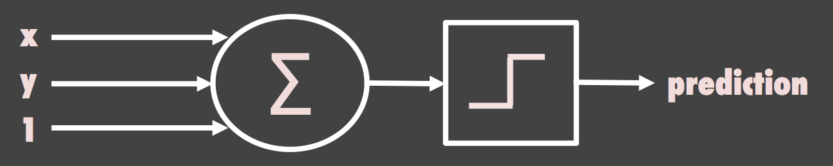
The perceptron takes a set of inputs (here, the x and y coordinates of each point, plus a fixed bias input of 1) and computes a weighted sum. Each input is multiplied by a corresponding weight, and the results are added together. This sum is then passed through an activation function: if the sum is positive, the output is +1; if negative, the output is -1. This is a simple threshold or step function.
The learning algorithm is called the delta rule. For each training point:
- Feed forward. Compute the weighted sum and apply the activation function to get the perceptron's prediction.
- Calculate error. Compare the prediction to the actual answer (is the point really above or below the target line?).
- Update weights. Adjust each weight by an amount proportional to the input, the error, and a small learning rate.
The weight diagram below the canvas shows the three weights updating in real time as the perceptron trains. The x and y weights control the slope of the current hyperplane, while the bias weight shifts it up or down.
Why It Matters
The perceptron convergence theorem, proved by Rosenblatt, guarantees that if a set of data is linearly separable (meaning a straight line can perfectly divide the two classes), the perceptron will find that line in a finite number of steps. This is a remarkable property: you don't need to tell it what the line looks like; you just show it examples and it figures it out.
However, a single-layer perceptron can only solve linearly separable problems. In 1969, Marvin Minsky and Seymour Papert published Perceptrons, a book that proved the single-layer perceptron cannot learn the XOR function (a problem where the two classes can't be separated by a single straight line). This result contributed to the first "AI winter," a period of reduced funding and interest in neural network research.
Beyond the Single Layer
The limitations identified by Minsky and Papert were eventually overcome by multi-layer perceptrons (MLPs), which add one or more hidden layers between the inputs and output. Combined with the backpropagation algorithm (popularized in the 1980s by Rumelhart, Hinton, and Williams), these deeper networks can learn nonlinear decision boundaries and solve problems like XOR.
The single-layer perceptron you see here is the building block on which all modern neural networks rest. Every neuron in a deep learning model is, at its core, doing the same thing: computing a weighted sum of inputs, passing it through an activation function, and adjusting its weights based on error signals. The difference is just a matter of scale and depth.