An Bound for the KLS Constant
Abstract: The Kannan--Lovász--Simonovits (KLS) conjecture asks whether every isotropic log-concave probability measure on has a Cheeger constant bounded below by a universal positive constant. We prove that for a universal constant $C>0$, resolving the KLS conjecture. We also prove that $C_P(μ)\le C'$ for every isotropic log-concave probability measure on , with a universal constant $C'>0$.
Paper Prompts
Sign up for free to create and run prompts on this paper.
Top Community Prompts
Explain it Like I'm 14
1. What is this paper about?
This paper studies the Kannan–Lovász–Simonovits (KLS) conjecture, a famous problem in mathematics about the shapes of high-dimensional objects and how quickly random processes move through them.
The paper claims to prove that a certain quantity, called the KLS constant, is always bounded by one fixed number, no matter:
- how many dimensions there are,
- which suitable probability distribution is used, or
- which test function is studied.
In simple terms, the paper says that high-dimensional, reasonably “well-shaped” probability distributions cannot have extremely narrow bottlenecks.
2. What questions are the researchers asking?
The main question is:
Can every well-balanced, log-concave probability distribution spread out in a controlled way, even in very high dimensions?
More specifically, the researchers want to show that for every such distribution and every function ,
where is a universal constant.
This formula compares two things:
- Variance: how much the values of change.
- Gradient energy: how quickly changes from place to place.
The result says that if a function changes greatly overall, then it must also change noticeably nearby. Its total variation cannot be large while its local changes remain tiny.
The paper also asks whether this result can be converted into a geometric statement: does every such distribution have a sufficiently large “boundary” between its different regions?
3. What ideas and methods are used?
Important definitions
A probability distribution is log-concave if its graph has no unexpected bumps or separated peaks. A simple example is a bell-shaped distribution. More generally, its mass is concentrated in a convex, well-behaved way.
A distribution is isotropic when it is centered at zero and has been scaled so that it spreads equally in every direction. It is like placing an object so that its center is at the origin and its average width is normalized.
The Poincaré constant measures how difficult it is for a function to vary across the distribution. The smaller this constant is, the more tightly controlled the variation is.
The Cheeger constant measures how easy it is to cut the distribution into two large pieces. If a shape has a narrow waist, it has a small Cheeger constant. If every possible cut has a large boundary, it has a large Cheeger constant.
These two constants are closely related:
- good boundary connections imply good control of variance;
- good variance control implies there are no serious bottlenecks.
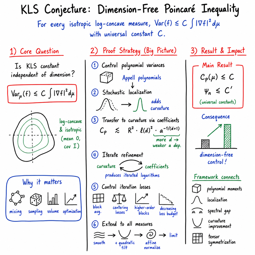
The overall strategy
The proof uses several advanced mathematical tools, but the basic plan can be described in stages.
Step 1: Study polynomials first
Instead of immediately studying every possible function, the researchers first study polynomials, such as
Polynomials are useful because they can be broken into pieces of different degrees, much like a complicated sound can be broken into simpler musical notes.
The paper constructs special polynomial pieces, called Appell polynomials, that are adapted to the probability distribution. The researchers then estimate how much these polynomials can fluctuate.
A major ingredient is an inequality controlling quadratic expressions such as
This says, roughly, that even complicated quadratic measurements of the random point cannot fluctuate too wildly.
Step 2: Use localization
The proof uses a method called stochastic localization.
An everyday analogy is slowly shining a flashlight on a complicated object. As the process continues, the original distribution is transformed into simpler “posterior” distributions. The researchers track how the shape and covariance of these distributions change.
This allows them to study a difficult high-dimensional problem through a sequence of more controlled problems.
Step 3: Connect polynomial control to curvature
The researchers first consider smooth distributions whose density has a definite amount of curvature. Curvature here means that the distribution bends upward enough to prevent it from becoming too flat or developing a dangerous bottleneck.
They show that good estimates for polynomials lead to good estimates for all functions. This is similar to learning that a machine works correctly on many standard test cases and then proving that it works correctly for every input.
Step 4: Repeatedly improve the estimates
At first, the method gives bounds involving logarithms, such as
where measures the amount of curvature.
The researchers then repeat their improvement process. Each repetition replaces a large quantity by its logarithm, then by the logarithm of that logarithm, and so on. This produces iterated logarithms, written informally as .
The function counts how many times one must apply a logarithm before a number becomes small. Even for very large numbers, this count grows extremely slowly.
Step 5: Prevent the repeated improvements from becoming too expensive
Repeating an argument many times can create extra errors. The paper uses “blocks” of steps and assigns smaller error allowances to later blocks.
The error allowances decrease geometrically, like
Because these errors add up to a finite amount, the total cost remains controlled.
Finally, the researchers use approximation to remove the smoothness assumptions. This extends the result to all isotropic log-concave distributions, including distributions with rough edges or bounded support.
4. What are the main findings?
The paper claims two main results.
A universal Poincaré bound
For every isotropic log-concave probability distribution ,
where is a universal constant.
This means the bound does not grow with the dimension. A distribution in one million dimensions is controlled just as well, in this sense, as one in two dimensions.
A universal KLS bound
The paper also claims
for every dimension , where is the worst possible reciprocal Cheeger constant among isotropic log-concave distributions in that dimension.
This is presented as a solution to the KLS conjecture.
Why this is important
Before this claimed result, the best known bounds became larger as the dimension increased, although researchers had gradually improved them. The paper says that all dependence on dimension can finally be removed.
This is important because these constants control how quickly certain random walks mix, or become close to their intended distribution.
5. Why could this research matter?
The KLS conjecture is connected to several practical mathematical algorithms. A dimension-independent bound could improve methods for:
- sampling random points from complicated convex shapes,
- estimating the volume of high-dimensional objects,
- computing integrals involving log-concave distributions,
- solving some convex optimization problems,
- putting shapes into a useful normalized position.
For example, imagine a random explorer walking inside a huge, oddly shaped room. If the room has a very narrow passage, the explorer may take a very long time to reach every part of it. The KLS result says that for the class of shapes studied here, such extreme bottlenecks cannot occur after proper normalization.
In short, the paper claims to show that high-dimensional log-concave distributions are more uniformly connected than previously proved. If the proof is correct and accepted by the mathematical community, it would settle a major open problem and could lead to faster and more reliable algorithms for high-dimensional geometry and probability.
Knowledge Gaps
Knowledge gaps, limitations, and open questions
- The central proof cannot be independently verified from the provided text. The paper presents an extensive proof roadmap and cites many lemmas and propositions, but the supplied manuscript ends during the preliminary stochastic-calculus section and does not include the sections containing the main technical proofs.
- The claimed universal constants are not made explicit. The results use multiple unspecified constants, including the constants in the polynomial estimates, curvature comparison, block estimates, and repetition-cost argument. It remains unclear whether these constants can be tracked effectively or whether the proof yields a usable numerical bound for the KLS constant.
- The dependence of constants across nested iterations is not fully transparent. The argument repeatedly composes inner logarithmic refinements, outer height reductions, block orders, cutoffs, and starting depths. A complete verification is needed that all dependencies remain dimension-free and that no hidden dependence on , , the polynomial degree, or the iteration depth re-enters through intermediate estimates.
- The validity of the high-order block estimates is a critical unresolved point. The final dimension-free conclusion relies on centering losses of order for arbitrary odd block orders and on uniform control of the associated derivative families. The supplied overview does not establish these estimates or clarify the regularity and integrability conditions required for them.
- The near-unit-cost repetition argument requires further justification. The proof replaces a fixed multiplicative loss per outer iteration by factors of the form and assigns geometrically decreasing loss budgets. It remains to verify rigorously that the enlarged cutoffs, starting depths, and coefficient ranges caused by small are controlled uniformly throughout the infinite family of potential repetitions.
- The termination argument is qualitative rather than quantitative. Repeated application of the shifted log-star map is shown only schematically to reach a bounded range. The resulting number of repetitions and the associated thresholds should be quantified carefully, especially when inserted into the cutoff and depth-selection arguments.
- The passage from polynomial variance bounds to the full Poincaré inequality is not fully elucidated. The paper establishes estimates for Appell-type polynomials and uses spectral and inverse-gradient constructions, but the precise density or approximation argument showing that these estimates control arbitrary locally Lipschitz functions with finite Dirichlet energy is not available in the supplied text.
- The role of Appell-polynomial nonorthogonality remains potentially delicate. The argument explicitly uses Minkowski’s inequality rather than orthogonality, but it is not clear from the overview whether the resulting coefficient accumulation is sharp enough at every iteration or whether cross-degree correlations could introduce additional losses.
- The localization argument’s uniformity over posterior measures needs complete verification. The proof applies polynomial and curvature estimates to affinely normalized stochastic-localization posteriors. It remains necessary to verify that these posteriors satisfy all required assumptions—centeredness, covariance upper bounds, curvature lower bounds, moment conditions, and regularity—uniformly up to the stopping times used.
- The treatment of nonsmooth and bounded-support log-concave measures is dependent on an approximation theory that is only asserted. The final extension uses regular isotropic approximation and Poincaré-limit lemmas, but the preservation of isotropy, covariance control, normalization, and convergence of the relevant functional constants requires detailed proof.
- The theorem’s formulation for arbitrary locally Lipschitz functions needs sharper domain clarification. The result asserts that finite Dirichlet energy implies membership in , but the exact Sobolev closure, representative choice, and boundary treatment for measures supported on nonsmooth convex bodies are not established in the provided material.
- The use of first positive eigenfunctions is not obviously available in every intermediate setting. The curvature argument invokes a first positive eigenfunction of a weighted diffusion operator with compact resolvent. It remains to verify compactness of the resolvent, discreteness of the spectrum, and existence of an eigenfunction for every smooth uniformly log-concave measure and every posterior considered.
- The proof depends substantially on Letwin’s quadratic-form inequality without addressing its scope or possible sharpness. The argument assumes the stated inequality for all isotropic log-concave measures and uses it as the base of a high-degree induction. It remains open whether the exact constant or form of this inequality is necessary, and whether weaker or more general quadratic-form estimates would suffice.
- The affine-covariant version is stated but not developed in detail. The paper notes that the conjecture should scale with , but it does not fully explain how the proof transforms under arbitrary affine maps or whether the intermediate covariance-at-most- estimates yield the optimal covariance dependence.
- The result is nonconstructive from an algorithmic perspective. Although the introduction emphasizes implications for sampling, integration, and convex optimization, the proof does not provide an explicit algorithm for estimating the constant, identifying the relevant localization parameters, or converting the theorem into concrete mixing-time bounds.
- No lower-bound or extremal analysis is provided. The paper establishes an upper bound but does not identify distributions that are close to extremizing the universal Poincaré or Cheeger constant, nor does it determine whether Gaussian, product, unconditional, or specially constructed measures govern the worst case.
- The sharpness of the universal bound is unknown. Even if the KLS conjecture is resolved, the optimal universal constants for and remain undetermined, as does the asymptotic behavior of the supremum over dimensions.
- The proof does not clarify whether its techniques extend beyond log-concavity. It remains open whether analogous polynomial-localization and iterative-curvature methods apply to broader classes such as approximately log-concave, weakly log-concave, or measures satisfying only functional moment conditions.
- Stability under perturbations is unexplored. The paper does not determine how the bound changes for distributions that are close to isotropic log-concave measures in total variation, Wasserstein distance, covariance distance, or density ratios.
- The relationship between the Poincaré and Cheeger conclusions is not optimized. The Cheeger bound is obtained through a general comparison that introduces universal losses. It is unknown whether the method can directly establish a sharper isoperimetric inequality or improve the constants in the conversion from to .
- The manuscript contains apparent notation and LaTeX inconsistencies that require resolution before the proof can be assessed reliably. Examples include malformed definitions of operators and norms, missing braces in several equations, inconsistent theorem labels, and apparent typographical errors in stochastic-integral and covariance expressions. These issues may be purely transcriptional, but they currently obstruct formal verification.
Practical Applications
Immediate Applications
The paper’s central result is a dimension-free Poincaré inequality for isotropic log-concave measures, equivalently an KLS bound. The applications below are immediate at the level of mathematical guarantees and algorithm design, although practical deployment still requires implementation-specific constants and numerical validation.
- Faster theoretical guarantees for sampling from convex bodies (software, optimization, computational geometry)
- Potential workflow: approximately isotropize a convex body or target distribution, run a log-concave random walk, and use the universal Poincaré/Cheeger bound to certify convergence.
- Practical outputs: sampling libraries for convex polytopes, posterior distributions, and constrained optimization problems with provable convergence rates.
- Dependencies: the theorem assumes log-concavity and isotropic or suitably normalized covariance; the hidden universal constants may be too large for practical runtime estimates.
- Improved algorithms for volume computation and log-concave integration (computational geometry, statistics)
- Potential tools: randomized volume estimators, partition-function estimators, and integration routines for log-concave densities.
- Use cases: computing volumes of high-dimensional polytopes, estimating normalization constants, and evaluating expectations under truncated or constrained distributions.
- Dependencies: efficient approximate isotropic rounding is still required, and discretization, oracle-access, and numerical-error assumptions must be handled separately.
- More robust convergence analysis for convex optimization methods (optimization, machine learning)
- Potential workflow: use a log-concave sampling subroutine inside simulated annealing or Bayesian optimization, with dimension dependence no longer arising from the worst-case KLS factor.
- Potential products: certified samplers for constrained convex optimization and software packages that automatically normalize convex feasible regions.
- Dependencies: the theorem concerns log-concave measures, not arbitrary nonconvex objectives; computational overhead for evaluating densities and gradients remains relevant.
- Dimension-robust concentration and uncertainty quantification for log-concave models (statistics, data science, finance, engineering) A Poincaré inequality bounds the variance of any sufficiently regular observable by its average squared gradient:
This can be used to control sensitivity of statistics, simulation outputs, and risk functionals under log-concave uncertainty models. - Potential workflow: represent uncertain parameters with a log-concave distribution, compute or bound , and obtain a dimension-independent variance certificate. - Examples: uncertainty propagation in engineering systems, sensitivity analysis for Bayesian posteriors with log-concave likelihoods, and variance bounds for convex risk measures. - Dependencies: the observable must have finite Dirichlet energy, and the relevant distribution must genuinely be log-concave after normalization.
- Improved analysis of Bayesian sampling for log-concave posteriors (statistics, healthcare, finance)
- Potential tools: posterior samplers with automatic covariance normalization, mixing diagnostics based on conductance, and dimension-robust error bounds for posterior expectations.
- Dependencies: posterior log-concavity is essential; multimodal or non-log-concave posteriors are outside the theorem’s scope. Approximate rather than exact isotropy introduces additional condition-number dependence.
- Dimension-free control of polynomial observables (academia, scientific computing, applied probability)
- Potential workflow: expand a polynomial observable into centered Appell components and apply the paper’s tensor variance estimates without paying a dimension-dependent factor.
- Applications: moment bounds, approximation theory, stochastic simulation, and analysis of high-dimensional random vectors.
- Dependencies: the polynomial degree and tensor norms still affect the bound, even though the ambient dimension does not.
- A reusable proof framework for extending smooth results to nonsmooth log-concave measures (academia, mathematical software)
- Potential use: adapt the approximation-and-limit strategy to other functional inequalities or diffusion estimates for nonsmooth convex potentials.
- Dependencies: transferring the framework requires verifying the relevant compactness, Sobolev, and approximation properties in the new setting.
Long-Term Applications
These applications depend on independently verifying the paper’s proof, extracting usable numerical constants, designing scalable implementations, or extending the theorem beyond its stated assumptions.
- Near-optimal high-dimensional sampling platforms (software, computational statistics, AI)
- Possible product: a “log-concave sampling engine” supporting polytopes, exponential-family posteriors, and constrained machine-learning models.
- Required development: explicit constants, discretization guarantees, adaptive isotropization, parallel implementations, and empirical benchmarks.
- Key assumption: target distributions must remain log-concave or be decomposable into efficiently handled log-concave components.
- Scalable Bayesian inference in high-dimensional healthcare and finance (healthcare, finance, econometrics)
- Potential applications: probabilistic imaging reconstruction, survival models, portfolio-risk estimation, and high-dimensional generalized linear models.
- Required development: sparse-gradient and Hessian methods, distributed sampling, handling data-access costs, and robust diagnostics for approximate isotropy.
- Limitations: realistic models often contain nonconvex likelihoods, discrete variables, latent mixtures, or multimodal posteriors.
- Improved volume and partition-function estimation for scientific and industrial design (materials, robotics, energy, computational geometry)
- Potential tools: certified estimators for feasible-region volume, entropy, and partition functions; uncertainty-aware design-space mapping.
- Required development: efficient oracle implementations, numerical stability, and methods for bodies described implicitly by simulations rather than explicit inequalities.
- Key dependency: the feasible set must be convex or adequately approximated by a convex body.
- Faster randomized motion planning in convex or locally convex configuration spaces (robotics)
- Potential workflow: isotropize a convex configuration-space region, sample configurations with a log-concave random walk, and use the samples for coverage or planning.
- Required development: geometry-aware samplers, collision-checking integration, and extensions to manifolds or nonconvex free spaces.
- Limitation: general robot configuration spaces are highly nonconvex, so the theorem would primarily apply to convex subproblems or local relaxations.
- Dimension-robust uncertainty propagation for engineering and energy systems (energy, climate, aerospace, control)
- Potential workflow: calculate or bound sensitivities of a simulator output and convert them into variance bounds.
- Potential products: safety-certification modules, robust design tools, and sensitivity-analysis dashboards.
- Required development: automatic differentiation through simulators, treatment of nonsmooth outputs, and conservative but computable gradient bounds.
- New functional inequalities and mixing results beyond log-concavity (academia)
- Possible extensions: approximately log-concave measures, measures with weakly convex potentials, structured nonconvex distributions, or distributions satisfying other concentration properties.
- Potential outcome: improved Poincaré, Cheeger, log-Sobolev, or transportation inequalities under weaker assumptions.
- Dependencies: the present argument relies strongly on convexity, localization stability, curvature control, and regular approximation; these components may fail in non-log-concave settings.
- Automated theorem-to-algorithm pipelines for convex probability (formal methods, mathematical AI)
- Potential tool: software that takes assumptions on a convex potential and produces certified variance, conductance, or mixing bounds.
- Required development: explicit constants, machine-checkable proofs, formalization of stochastic localization, and interfaces to numerical optimization software.
- Limitation: the paper’s universal-constant notation is qualitative; practical certification requires replacing bounds with explicit computable quantities.
- Improved theoretical foundations for high-dimensional learning under convex uncertainty (machine learning, education technology, decision systems)
- Potential workflow: use gradient sensitivity of a prediction or loss function together with the Poincaré inequality to bound variability across parameter or data perturbations.
- Required development: connect the measure-theoretic result to empirical-process bounds, finite-sample learning theory, and stochastic optimization.
- Limitation: the result is not itself a generalization theorem and does not automatically address data dependence, model misspecification, or nonconvex neural-network losses.
Glossary
- Affine normalization: Rescaling and translating a measure by an invertible affine transformation to obtain a standardized form, such as isotropic position. “After affine normalization, the posterior has curvature at least a constant multiple of .”
- Appell polynomials: Polynomial sequences characterized by a generating function and derivative identities, generalized here to multivariate probability measures. “We write the multivariate Appell polynomials associated with ~\cite{a04} as symmetric tensor-valued polynomials .”
- Brascamp--Lieb inequality: A functional inequality bounding variance by a weighted gradient energy using the inverse of a curvature matrix. “The following form of the Brascamp--Lieb inequality converts the matrix of this quadratic term into a weighted Poincaré inequality.”
- Cheeger constant: A measure’s isoperimetric constant, defined through the boundary measure of sets relative to their smaller measure. “The Cheeger constant of and its reciprocal are”
- Cheeger--Buser inequality: A comparison relating the Cheeger constant to the spectral or Poincaré constant in both directions. “For full-dimensional log-concave measures, Cheeger’s inequality and the reverse Cheeger--Buser inequality show that and are comparable up to universal factors.”
- Conductance: A measure of how readily a Markov chain moves between regions of its state space, often controlling mixing time. “Bounds on the KLS constant control conductance and mixing times, and thereby the complexity of sampling, volume computation, and log-concave integration.”
- Covariance operator: A matrix-valued operator describing the second-moment structure of a random vector. “The covariance dependence is necessary: testing Eq.~\eqref{eq:introduction_poincare} against linear functions gives $C_P(\mu)\geq\|\Sigma\|_{\mathrm{op}$.”
- Curvature lower bound: A uniform lower bound on the Hessian of a potential function, indicating strong convexity. “The proof begins with smooth, uniformly log-concave measures of covariance at most .”
- Dirichlet energy: The integral of the squared gradient of a function with respect to a measure. “for every locally Lipschitz function with finite Dirichlet energy”
- Dyadic: Relating to powers of two, often used to organize scales or degrees. “then, for every dyadic ,”
- Eigenfunction: A function mapped to a scalar multiple of itself by an operator. “choose an eigenfunction corresponding to its first positive eigenvalue”
- Extended-real-valued convex function: A convex function allowed to take the value , commonly encoding constraints or support restrictions. “where is an extended-real-valued convex function and may equal outside the support.”
- Gaussian localization: A stochastic procedure that progressively modifies a measure using Gaussian observations or tilts. “For the dimensional estimate, we return to Gaussian localization.”
- Gronwall’s inequality: An inequality that bounds solutions of integral or differential inequalities through exponential growth estimates. “We repeatedly apply Gronwall’s inequality to the derivative energies along localization.”
- Hilbert--Schmidt norm: The square root of the sum of squared matrix or tensor entries, equivalent to the Frobenius norm for matrices. “where $\|\cdot\|_{\mathrm{HS}$ is the Hilbert--Schmidt norm.”
- Hessian: The matrix of second-order partial derivatives of a scalar function. “The weighted Bochner identity expresses the squared norm of the weighted Laplacian applied to a function as the sum of a Hessian term and a curvature term.”
- Isoperimetric statement: A result relating the boundary size of a set to the measure of the set and its complement. “Thus the conjecture is equivalently a dimension-free isoperimetric statement.”
- Isotropic measure: A probability measure with zero mean and identity covariance matrix. “We call isotropic when its mean is zero and its covariance is the identity”
- Itô’s formula: A stochastic-calculus analogue of the chain rule for functions of stochastic processes. “For It^o's formula, the product rule, and the isometry below”
- KLS constant: A dimension-dependent supremum of reciprocal Cheeger constants over isotropic log-concave measures. “let be the supremum of the reciprocal Cheeger constant over all isotropic log-concave probability measures on .”
- Log-concave measure: A measure whose density has a log-concave form, or equivalently satisfies a multiplicative convexity inequality on sets. “The Kannan--Lovász--Simonovits (KLS) conjecture asks whether every isotropic log-concave probability measure on has a Cheeger constant bounded below by a universal positive constant.”
- Log-star function: The number of repeated logarithms needed to reduce a value to a bounded size. “Writing for the least number of successive natural logarithms needed to bring to at most one”
- Martingale: A stochastic process whose conditional expected future value equals its present value. “A bounded continuous local martingale is a martingale.”
- Minkowski inequality: A triangle inequality for norms of sums, including sums of vector-valued random variables. “The polynomial estimates use the following forms of Minkowski's and Bessel's inequalities.”
- Poincaré constant: The smallest constant bounding variance by integrated squared gradient. “Write for the Poincaré constant of ”
- Posterior measure: A probability measure updated after incorporating information from observations or a stochastic process. “We use this inequality to bound the third-moment tensors that govern covariance fluctuations during localization”
- Quadratic-form inequality: A variance estimate for expressions of the form . “A key estimate controlling fluctuations of the posterior covariance is Letwin's quadratic-form inequality”
- Rayleigh characterization: A variational description of an operator’s smallest positive eigenvalue through a quotient of energies. “Expansion in this basis gives the Rayleigh characterization of its least positive eigenvalue on .”
- Reciprocal Cheeger constant: The inverse of the Cheeger constant, used in the KLS formulation. “The Kannan--Lovász--Simonovits (KLS) conjecture asks whether every isotropic log-concave probability measure on has a Cheeger constant bounded below by a universal positive constant.”
- Spectral gap: The smallest positive eigenvalue of an operator governing variance decay or mixing. “Since the initial energy is , we can rule out a spectral gap that is too small and obtain the stated bound on .”
- Spectral subspace: A subspace spanned by eigenvectors whose eigenvalues lie in a specified range. “On a spectral subspace where with , it also gives $\|H^{-1/2}\|_{\mathrm{op}\le\lambda^{-1/2}$.”
- Stochastic Fubini theorem: A result permitting interchange of spatial or parameter integration with stochastic integration under square-integrability conditions. “We also need to interchange a spatial integral with a stochastic integral.”
- Stochastic localization: A stochastic process that transforms a probability measure into evolving posterior measures while controlling their geometric properties. “Subsequent progress used thin-shell concentration~\cite{bobkov_2007_isoperimetric,guedon_milman_2011} and Eldan's stochastic localization method~\cite{eldan_2013}.”
- Supermartingale: A stochastic process whose conditional expected future value is no greater than its current value. “A nonnegative continuous local supermartingale with $\E Z_0<\infty$ is a supermartingale”
- Tensor contraction: The operation of summing over matching tensor indices to reduce tensor order. “Differentiating once contracts with .”
- Thin-shell concentration: Concentration of the norm of a high-dimensional random vector in a narrow shell around its typical radius. “Subsequent progress used thin-shell concentration~\cite{bobkov_2007_isoperimetric,guedon_milman_2011}”
- Uniformly log-concave measure: A log-concave measure whose potential has a Hessian bounded below by a positive multiple of the identity. “The proof begins with smooth, uniformly log-concave measures of covariance at most .”
- Weighted Bochner identity: An identity decomposing the squared weighted Laplacian into Hessian and curvature contributions. “The weighted Bochner identity expresses the squared norm of the weighted Laplacian applied to a function as the sum of a Hessian term and a curvature term.”
- Weighted Laplacian: A differential operator adapted to a weighted measure, combining the ordinary Laplacian with drift from the measure’s potential. “For the operator arguments in Section~\ref{sec:analytic_foundations}, we use two standard facts about Sobolev spaces”

