Probe-Space Preconditioning for Fast and Stable Zero-Order Training
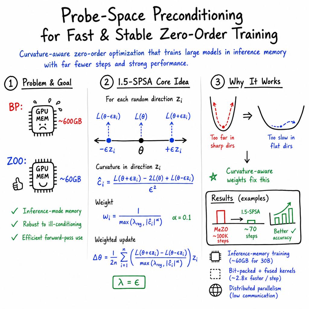
Abstract: Backpropagation (BP) dominates deep learning but imposes a massive memory tax. For example, training OPT-30B with Adam requires 600GB of GPU memory (assuming batch size 8 and sequence length 2048). Alternatively, zero-order optimization (ZOO) trains in inference-mode (requiring only 60GB for the same model): no stored activations, no gradients, and no optimizer states. However, ZOO convergence has lagged behind BP. In this work, we evaluate two methods to close this gap. First, we show that reallocating training compute budget from many steps to large effective batch sizes with many perturbations (or probes) but fewer steps, allows 1SPSA (Spall, 1992) to outperform zero order methods like MeZO (Malladi et al., 2023) with less training compute. Next, we introduce 1.5-SPSA, adding a single "clean" forward-pass per step to 1SPSA to calculate a cheap diagonal preconditioner in probe-space, which improves convergence rate and convergence by down-weighting high curvature directions. Benchmarking on 6 post-training datasets on both Qwen3 and OPT model families, we show that 1.5-SPSA achieves State-of-the-Art results over previous ZOO solvers with much less optimization steps. For example, we train OPT-13B (for direct comparison to MeZO) and find 1.5-SPSA achieves +3.1% accuracy on SST-2 over both MeZO and BP in only 70 steps vs. MeZO's 100,000 steps. Finally, we combine an 8-bit-packing random generator, triton fused unpack/apply kernels, and distributed parallelism to achieve fast and stable training of models as large as OPT-30B in-place on commodity GPUs (e.g. A100).
Paper Prompts
Sign up for free to create and run prompts on this paper.
Top Community Prompts
Explain it Like I'm 14
1. What is this paper about?
This paper presents a new way to train very large neural networks while using much less computer memory.
Most modern AI models are trained with backpropagation, a method that calculates exactly how every model parameter should change. Backpropagation works well, but it needs to save many intermediate calculations and extra information. For a very large model, this can require hundreds of gigabytes of GPU memory.
The paper studies a different approach called zero-order optimization, or ZOO. Instead of calculating exact gradients, ZOO tries small changes to the model and observes whether the result gets better or worse. The authors introduce an improved ZOO method called 1.5-SPSA.
Their goal is to make large-model training:
- Use much less memory
- Remain stable and accurate
- Finish with fewer training steps
- Work efficiently on ordinary high-end GPUs
2. What questions are the researchers asking?
The paper mainly investigates two questions:
- How should training calculations be distributed? Should the model take many small training steps, or should it use more tests and examples during each step and take fewer total steps?
- Can the method become more stable by noticing which directions are risky? Some changes to a model can make its error increase very quickly. The researchers ask whether they can detect these “sharp” directions and make smaller changes there.
The authors also ask whether their method can:
- Compete with older zero-order methods such as MeZO
- Sometimes match or beat backpropagation
- Work on different model families, including OPT and Qwen3
- Scale to models as large as OPT-30B
3. How does the research work?
Zero-order optimization: learning by trying small changes
Imagine trying to find the lowest point in a hilly landscape while blindfolded. You cannot see the slope, but you can take a small step in one direction and one in the opposite direction:
- If the first step makes things better, that direction may be useful.
- If the second step makes things better, move the other way.
- If both are bad, try a different direction.
In machine learning, the “height” of the landscape is the model’s loss, which measures how wrong the model is. Lower loss usually means better performance.
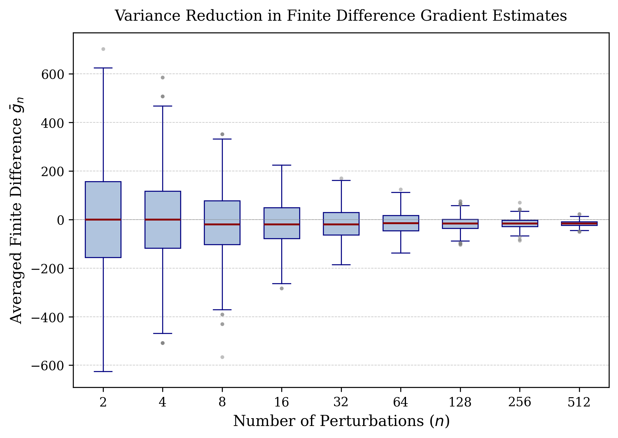
The researchers use random directions, called probes or perturbations, to test the model. This avoids calculating a full gradient, which would be very expensive for a model with billions of parameters.
1SPSA
The basic method is called 1SPSA, short for Simultaneous Perturbation Stochastic Approximation. It:
- Randomly chooses a direction.
- Changes the model slightly in that direction.
- Measures the loss.
- Changes the model slightly in the opposite direction.
- Measures the loss again.
- Uses the difference between the two measurements to decide how to update the model.
A useful feature is that the number of tests does not directly depend on the number of model parameters. This is important because LLMs may contain billions of parameters.
Changing the compute strategy
The researchers found that 1SPSA works better when it uses:
- More random probes per training step
- Larger effective batches of training examples
- Fewer total optimization steps
This is similar to asking many people for directions before making one large decision, rather than asking one person at a time and constantly changing course.
Using many probes also allows the work to be done in parallel on several GPUs.
1.5-SPSA and curvature
The new method, 1.5-SPSA, adds one extra “clean” measurement of the model at its current state.
This lets the method estimate curvature. Curvature describes how quickly the loss changes in a particular direction. A direction with high curvature is like a very steep or sharply curved part of a hill. Taking a normal-sized step there could cause the model to overshoot and become unstable.
1.5-SPSA therefore:
- Takes smaller steps in high-curvature directions
- Takes relatively larger steps in flatter directions
This is called preconditioning. In everyday language, it means adjusting the size of each step depending on how dangerous that direction appears to be.
The method only performs this adjustment in the random probe directions. It does not build or store the full curvature information for the entire model, which would require too much memory.
Engineering improvements
The authors also improve the computer implementation by:
- Storing random directions in a compact, bit-packed form
- Using specialized GPU operations to apply them quickly
- Sharing work across multiple GPUs
- Sending only small loss values between GPUs instead of large model data whenever possible
These changes help the method train large models while keeping memory close to what is needed just to run the model for prediction.
4. What did the researchers find?
Much lower memory use
For the example in the paper, training OPT-30B with backpropagation and Adam would require about 600 GB of GPU memory.
The zero-order approach requires about 60 GB, or roughly ten times less. This is because it does not need to store:
- Intermediate activations
- Gradients
- Adam’s additional optimizer information
This makes it possible to train very large models on fewer or less expensive GPUs.
Better use of training calculations
The experiments showed that 1SPSA performed better when the researchers used more probes and larger batches per step, rather than simply running many small steps.
For example, on the SST-2 language-understanding task with OPT-13B:
- MeZO reached about 91.4% accuracy
- 1SPSA reached about 94.2% accuracy
- 1.5-SPSA reached about 94.5% accuracy
The 1.5-SPSA result used only about 70 optimization steps, compared with about 100,000 steps for MeZO in the comparison described by the paper.
Improved stability
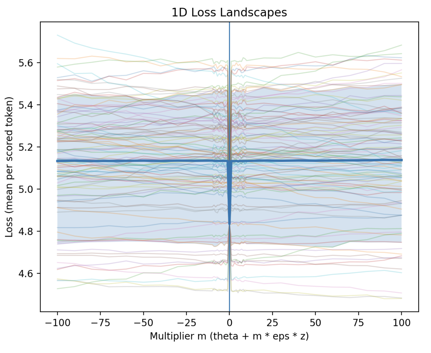
The curvature adjustment helped prevent training from becoming unstable. The method was especially helpful when the loss landscape was badly shaped, meaning that some directions were much steeper than others.
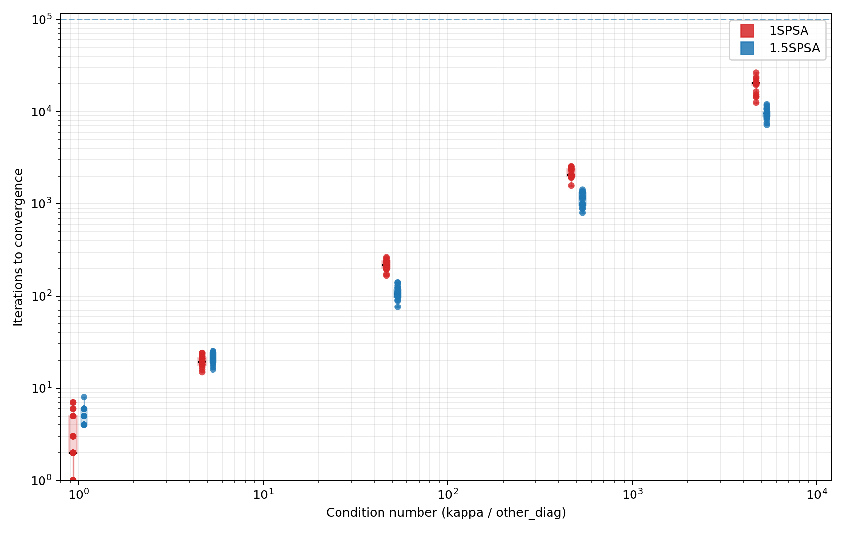
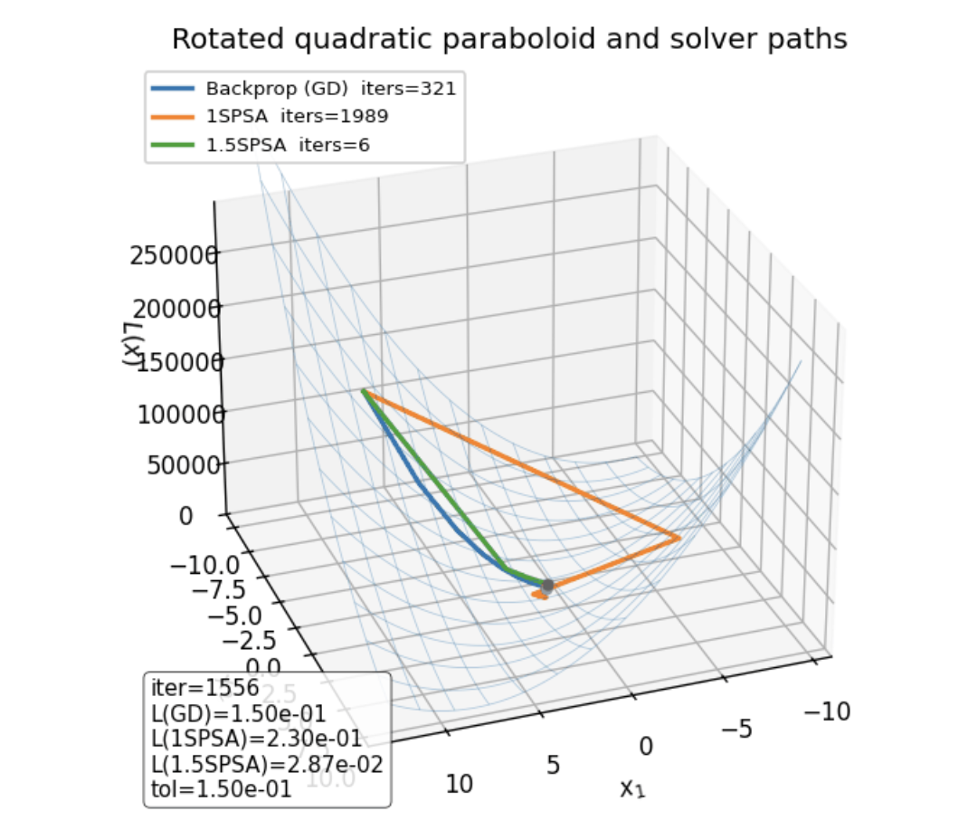
In a simple mathematical test, 1.5-SPSA became increasingly better than 1SPSA as the problem became more uneven. It sometimes needed up to about seven times fewer steps.
In experiments with difficult recurrent neural networks, 1.5-SPSA sometimes reached very low loss about six times faster than 1SPSA.
Results across different models and tasks
The method was tested on:
- OPT-13B
- OPT-30B
- Qwen3-1.7B
- Qwen3-8B
- Several language understanding tasks
- A tool-use task
- Synthetic mathematical problems
- Difficult recurrent neural networks
Overall, 1.5-SPSA usually performed better than standard 1SPSA and previous zero-order methods. In some tests, it also performed better than the backpropagation baselines.
However, the authors are careful to say that this does not prove that 1.5-SPSA is always better than backpropagation. The backpropagation methods were not fully retuned for every special experimental setup.
5. Why are these findings important?
Training large AI models is often limited by memory. A model may be able to run on a GPU for making predictions but not fit on that same GPU during training because training needs to save extra information.
This research suggests that models could be trained in a more memory-efficient way by:
- Avoiding stored gradients and activations
- Using many parallel model tests
- Adjusting step sizes based on local curvature
- Splitting the work across ordinary GPUs
The method could be useful for researchers or organizations that cannot afford very large GPU clusters. It may also make it easier to train large models directly on available hardware instead of relying on complicated memory-saving systems.
Conclusion
The paper introduces 1.5-SPSA, a method for training large neural networks without calculating traditional gradients.
Its main idea is simple:
- Try many small random changes to the model.
- Use the results to estimate which direction is helpful.
- Take smaller steps in directions that look dangerous or sharply curved.
- Use many tests at once so that fewer training steps are needed.
The experiments show that this approach can use about ten times less memory than backpropagation with Adam and can achieve strong accuracy with far fewer optimization steps than earlier zero-order methods.
The main limitation is that the method may require many forward tests and careful tuning of batch size, learning rate, and other settings. Even so, the research shows a promising path toward training very large AI models with less memory and lower hardware requirements.
Knowledge Gaps
Knowledge gaps, limitations, and open questions
- Limited breadth of empirical evaluation: The method is evaluated primarily on OPT and Qwen3 models, a small set of GLUE/SuperGLUE tasks, Stable ToolBench, synthetic paraboloids, and DNC overfitting. Its performance on other architectures, modalities, objectives, and large-scale generative tasks remains unknown.
- No comprehensive comparison with strongly tuned backpropagation: BP baselines are not optimized for the same large-batch, few-step regime as 1SPSA and 1.5-SPSA. It remains unresolved whether the proposed method retains an accuracy or compute advantage against carefully tuned BP methods using gradient accumulation, checkpointing, low-memory optimizers, or parameter-efficient fine-tuning.
- Unclear fairness of compute comparisons: Training cost is primarily measured by the number of forward passes, without consistently accounting for backward-pass cost, perturbation generation, parameter updates, communication, synchronization, kernel overhead, and model-memory transfers. The true end-to-end FLOP and wall-clock advantages over BP, MeZO, and other ZOO methods are therefore unresolved.
- Insufficient wall-clock benchmarking: The paper argues that perturbations can be parallelized, but provides limited systematic measurements of throughput, latency, scaling efficiency, energy consumption, and communication overhead across different numbers and types of accelerators.
- Scalability beyond OPT-30B is not established: Although the implementation is demonstrated up to OPT-30B, the memory, communication, and seed-regeneration costs for substantially larger models or longer sequence lengths are not quantified.
- Dependence on large parallel resources: The claimed speedups rely on distributing many perturbation evaluations across multiple GPUs. The method’s practicality on a single GPU, heterogeneous clusters, limited-bandwidth interconnects, or cloud environments with communication bottlenecks remains unclear.
- Sensitivity to hyperparameters is incompletely characterized: The method depends on , , , , batch size, number of perturbations, accumulation steps, and learning-rate scheduling. Only selected sweeps are reported, and the robustness of the method to untuned or automatically selected values is unresolved.
- The claimed generality of is not sufficiently supported: The conclusion that is consistently optimal is based on a limited set of architectures, tasks, and model sizes. Whether the optimal exponent varies with scale, loss type, batch size, perturbation distribution, or training stage remains open.
- The relationship between and lacks theoretical justification: The paper ties the learning rate to the perturbation radius, but does not establish when this coupling is optimal or how it behaves for nonquadratic, noisy, nonstationary objectives.
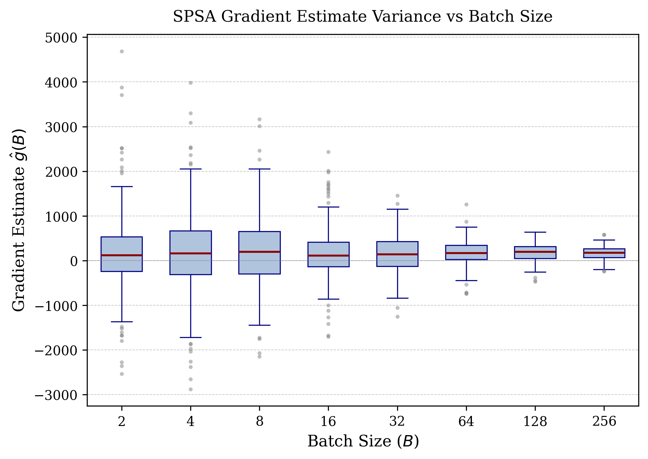
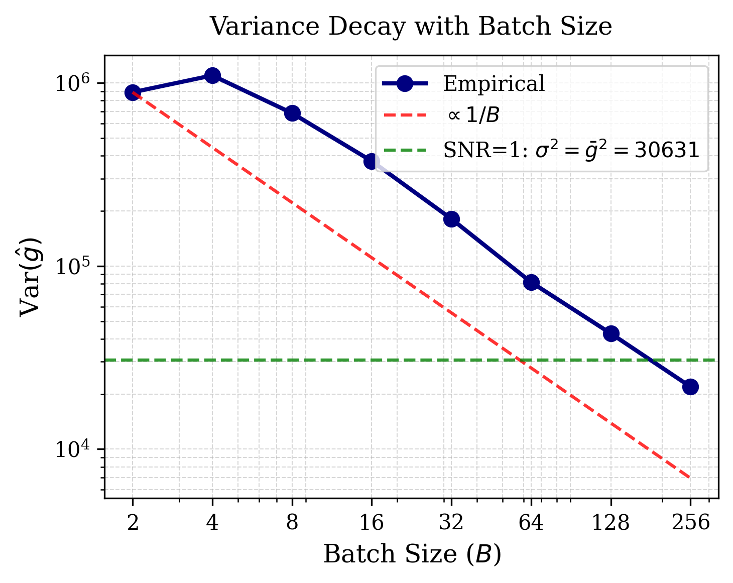
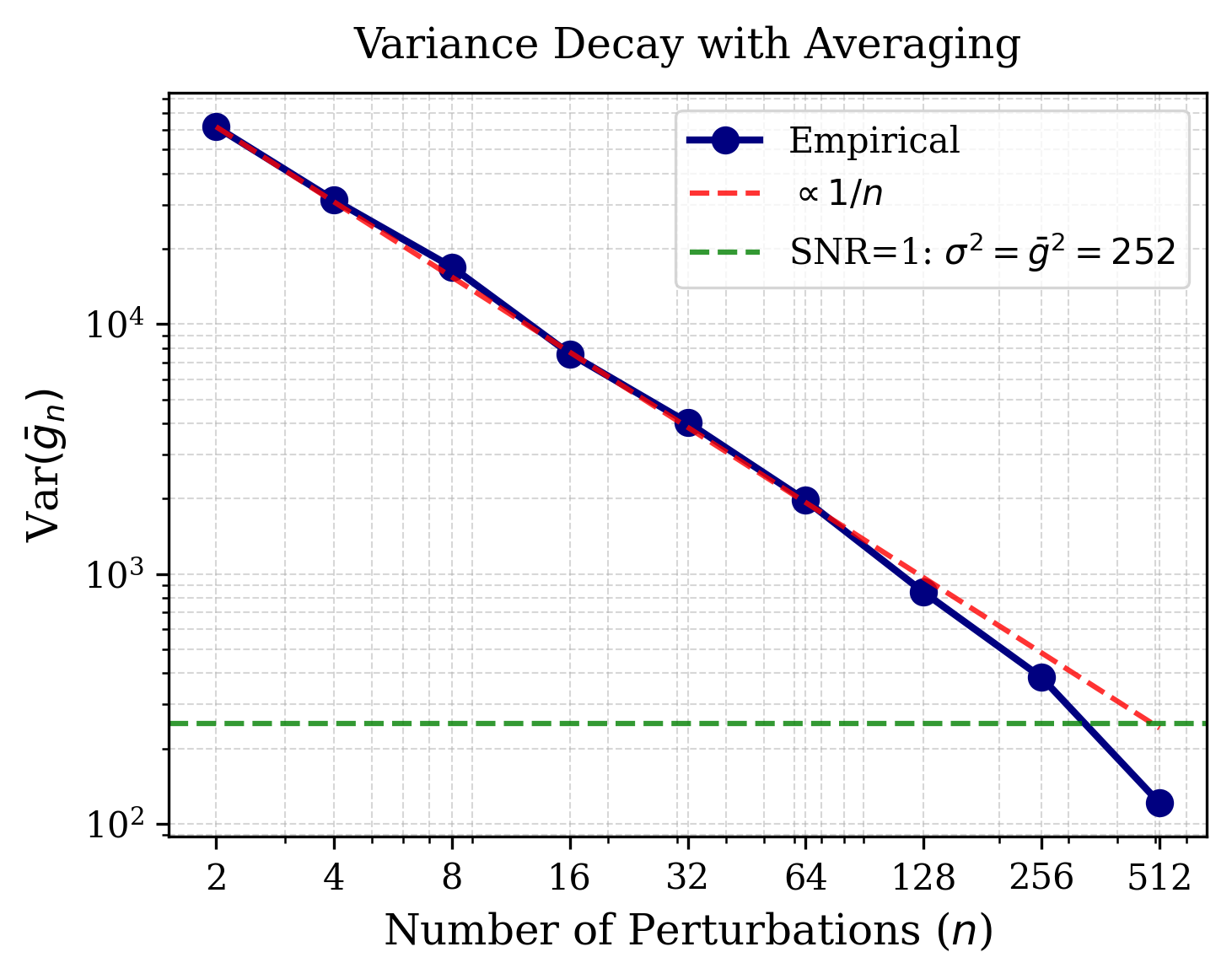
- No adaptive procedure for selecting batch size and perturbation count is demonstrated: The paper motivates using a signal-to-noise ratio near or above one, but does not provide or evaluate an online algorithm that estimates this quantity and adjusts resources during training.
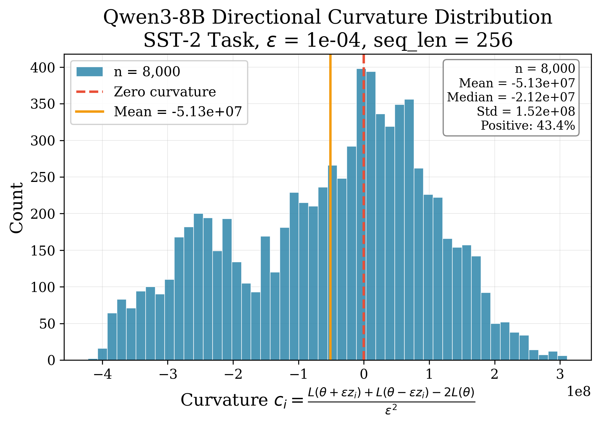
- Curvature estimates may be highly noisy: The three-point estimator uses stochastic minibatch losses, so combines true directional curvature with minibatch noise and finite-difference error. The paper does not quantify the estimator’s bias, variance, or reliability under different , batch sizes, and loss scales.
- The effect of loss normalization is unresolved: Directional curvature is not normalized across batches, perturbations, layers, or training stages. The paper identifies batch-normalized or relative curvature as a possible improvement but does not determine whether such normalization is necessary for robustness.
- The proposed probe-space preconditioning is not fully theoretically established: The argument based on a Johnson–Lindenstrauss extension suggests that curvature geometry may be preserved in random projections, but the conditions, approximation bounds, and practical implications for the highly nonconvex, stochastic neural-network setting are not fully derived or validated.
- The connection between probe-space curvature and parameter-space curvature remains unclear: It is not established when reweighting random directional probes approximates a useful parameter-space preconditioner, especially when the Hessian is anisotropic, indefinite, or has strong layerwise scale differences.
- Negative curvature is handled only through absolute values: The weighting uses , which removes the sign of curvature. The behavior of 1.5-SPSA near saddle points and in directions of strong negative curvature is not analyzed.
- The choice of regularization is underexplored: The experiments reportedly use , but the effect of this value, its dependence on loss scale, and principled ways to set it are not established.
- Finite-difference radius effects are not fully investigated: The method’s accuracy and stability may depend strongly on , especially as model scale, parameter magnitude, precision, and minibatch noise change. A comprehensive analysis of finite-difference bias versus stochastic variance is missing.
- Numerical stability at large model scale is not fully evaluated: The paper reports extremely large curvature values and uses low-precision inference-oriented kernels, but does not systematically analyze overflow, underflow, cancellation in central differences, or precision-related degradation.
- Random perturbation distributions are not compared: The method uses Rademacher probes, while structured, Gaussian, sparse, layerwise, orthogonal, or learned perturbations could alter variance and scaling. It remains unknown whether 1.5-SPSA’s gains depend specifically on Rademacher sampling.
- Layerwise parameter-scale mismatch remains insufficiently addressed: The paper notes that global perturbations can mix parameters with different scales, but does not compare 1.5-SPSA against layerwise or blockwise perturbation schemes such as LeZO, nor establish whether curvature weighting resolves this issue.
- Interaction with parameter-efficient fine-tuning is unresolved: Results for LoRA and prefix tuning are reported only for MeZO baselines. The memory, compute, and accuracy of 1SPSA and 1.5-SPSA applied to LoRA, adapters, prefix tuning, or selective parameter updates are not studied.
- Generalization beyond overfitting and post-training is uncertain: The DNC experiments measure steps to near-zero training loss, while the language-model experiments focus on short post-training tasks. The method’s behavior in long-horizon pretraining, reinforcement learning, instruction tuning, preference optimization, or distribution-shifted evaluation remains unknown.
- Generalization and catastrophic forgetting are not analyzed: The paper reports task accuracy but does not examine whether aggressive few-step updates and large perturbations harm performance on the original pretraining distribution or unrelated capabilities.
- Few random seeds and uncertainty estimates are reported: Most language-model results are presented as single accuracy values. Confidence intervals, variance across seeds, and statistical significance are needed to determine whether the reported gains are robust.
- Dataset-size and batch-composition effects are unclear: The large effective batches may repeatedly process limited post-training data. It is unresolved whether the gains arise from improved optimization, reduced sampling noise, repeated data exposure, or particular dataset sizes and class balances.
- The role of momentum and exploration is speculative: The paper attributes diminishing returns from larger batches and perturbation counts partly to the absence of momentum and the need to escape local minima, but does not test momentum-like alternatives that preserve the stated memory constraints.
- Late-training divergence is not fully solved: 1SPSA and, potentially, 1.5-SPSA can become unstable late in training. The proposed curvature weighting and plateau-based schedule do not completely resolve this, and the conditions causing divergence remain insufficiently characterized.
- No convergence theory is provided for the full neural-network algorithm: The paper does not establish convergence rates or stationarity guarantees for 1.5-SPSA with stochastic losses, adaptive curvature weights, finite perturbations, nonconvex objectives, and a coupled schedule.
- The effect of probe reuse and update ordering is unknown: The distributed implementation regenerates perturbations and applies updates sequentially on the coordinating rank. It is unclear whether ordering, seed assignment, asynchronous execution, or simultaneous aggregation changes the optimization trajectory.
- Communication and synchronization costs may become dominant: The method requires broadcasting model parameters after updates and coordinating perturbation evaluations. The crossover point at which communication outweighs the reduction in sequential forward computation is not determined.
- The claim of “no additional memory” is deployment-dependent: Although optimizer-state and activation memory are avoided, the implementation still requires model replicas across distributed ranks, temporary packed/unpacked perturbation buffers, and communication storage. Peak memory under realistic batch sizes and model configurations is not comprehensively reported.
- Robustness to stochastic or nondeterministic inference is not assessed: Dropout, quantization, generation randomness, data-loader nondeterminism, and hardware-level nondeterminism can corrupt finite-difference estimates. The method’s requirements for deterministic forward evaluations are not specified.
- Applicability to objectives with discrete or highly nonsmooth behavior is unclear: The analysis assumes that local finite differences provide useful directional information, but many post-training objectives involve discrete metrics, clipping, ranking, sampling, or discontinuous reward functions.
- The comparison with other ZOO and ES methods is incomplete: The study does not systematically compare against structured ZOO, variance-reduced methods, learned-subspace methods, evolution strategies, or memory-efficient adaptive zero-order optimizers under matched accuracy, FLOPs, wall-clock, and memory budgets.
- The source of the reported accuracy improvements is not isolated: It remains unclear how much of the gain comes from curvature weighting, larger learning rates, larger effective batches, more perturbations, fewer optimizer steps, or differences in data scheduling. A complete factorial ablation is needed.
- The claim of state-of-the-art ZOO performance may be benchmark-dependent: Results are concentrated on selected tasks and configurations, and broader evaluations are needed to establish whether the method consistently outperforms prior ZOO approaches rather than only under the chosen compute allocation.
- Long-term optimizer behavior is unknown: Experiments use fewer than roughly 300 optimization steps in the main post-training settings. Stability, convergence quality, and accumulated bias over substantially longer training runs have not been established.
- The effect of model quantization is unexplored: Since the method targets memory-constrained training and uses packed perturbations, compatibility with quantized model weights, quantized inference, and quantization-aware updates is an important unresolved question.
- Reproducibility is limited by incomplete implementation details: The paper does not fully specify all data-processing choices, seed handling, precision settings, hardware configurations, communication schedules, and hyperparameter-selection procedures needed to reproduce the reported results reliably.
Practical Applications
Immediate Applications
- Memory-constrained LLM post-training and fine-tuning — Software / AI infrastructure
- Deploy
1.5-SPSAas an optimizer for supervised fine-tuning, instruction tuning, classification, preference-oriented post-training, and tool-use training when GPU memory is the primary bottleneck. - The method can train models in inference mode without stored activations, gradients, or Adam-style optimizer states. The paper reports approximately
60 GBfor OPT-30B, compared with roughly600 GBfor BP+Adam under the stated configuration. - Potential product or workflow: a parameter-update engine integrated into PyTorch, Hugging Face Transformers, or distributed inference stacks, enabling post-training of large models on smaller GPU clusters.
- Dependencies and assumptions: effectiveness depends on the loss being measurable from forward passes, sufficient perturbation parallelism, careful tuning of learning rate , perturbation scale , batch size, and number of probes. The reported results focus primarily on post-training rather than unrestricted pretraining.
- Deploy
- Single-node or commodity-GPU model adaptation — AI infrastructure / cloud computing
- Use bit-packed Rademacher perturbations, fused Triton/CUDA kernels, and seed-based distributed generation to adapt models on limited hardware without storing full optimizer states.
- This is particularly relevant to organizations that have inference capacity but cannot afford large training clusters.
- Potential tool: an “inference-mode fine-tuning” service that reuses serving GPUs during low-demand periods.
- Dependencies and assumptions: model weights must fit across the available devices; communication of updated model parameters can become a bottleneck; the practical advantage increases when many GPUs can evaluate perturbations in parallel.
- Rapid few-step task adaptation for classification and tool-use models — NLP / enterprise AI
- The reported convergence in tens or hundreds of optimization steps can support fast adaptation to tasks such as sentiment classification, natural-language inference, question answering, and tool invocation.
- For example, the method could be used to update an enterprise model for a newly labeled customer-support taxonomy or a changing tool API without provisioning a large backpropagation training job.
- Dependencies and assumptions: the task must have a stable scalar loss and enough labeled data to produce a useful batch-level signal. Results on SST-2, GLUE/SuperGLUE tasks, and Stable ToolBench do not establish equivalent performance for every domain.
- Derivative-free optimization baselines for research and engineering — Academia / software
- Use
1SPSAand1.5-SPSAas practical baselines when gradients are unavailable, inaccessible, unreliable, or intentionally avoided. - The same workflow applies to black-box neural components, proprietary model APIs, simulators, and systems where only objective values can be queried.
- Potential tool: a benchmark suite comparing BP, MeZO, SPSA, evolutionary strategies, and perturbation-space preconditioners under matched forward-pass budgets.
- Dependencies and assumptions: objective evaluations must be sufficiently repeatable or the batch and perturbation sizes must be increased to overcome noise. Query cost, rather than GPU memory, may dominate in external API or simulator settings.
- Use
- Training recurrent models with difficult memory dynamics — Robotics / sequence modeling
- The DNC experiments suggest that perturbation-space curvature weighting can accelerate optimization of recurrent networks with external memory, including models that are difficult or expensive to train with backpropagation through time.
- Possible uses include learned controllers, episodic-memory models, sequence prediction, and differentiable memory modules.
- Dependencies and assumptions: the paper evaluates controlled overfitting stress tests rather than complete robotics deployments. Real-world recurrent tasks may introduce nonstationarity, long-horizon noise, and safety constraints that require additional stabilization.
- Efficient hyperparameter and architecture optimization — Academia / industrial R&D
- Apply the method to optimize models or components when the objective is available only through validation loss or task performance.
- Directional curvature estimates can identify unstable perturbations and support more aggressive search steps without maintaining a full Hessian or per-parameter optimizer state.
- Potential workflow: evaluate multiple perturbations in parallel, collect scalar validation losses, reweight high-curvature directions, and update the candidate configuration or model parameters.
- Dependencies and assumptions: continuous or smoothly varying parameters are more suitable than purely discrete design spaces; noisy validation metrics may require repeated evaluations and substantially larger budgets.
- Policy and public-sector model adaptation under hardware constraints — Government / education / nonprofit technology
- Public institutions could use inference-mode optimization to adapt open-weight LLMs to local legal, administrative, educational, or multilingual datasets without purchasing large accelerator clusters.
- This could reduce infrastructure costs and make local fine-tuning more feasible for universities, municipalities, and small research organizations.
- Dependencies and assumptions: the approach does not remove requirements for data governance, privacy protection, model evaluation, or secure distributed training. The paper does not directly evaluate regulated or high-stakes domains.
- Lower-memory experimentation in teaching and daily development — Education / individual developers
- Students and independent developers could experiment with large-model adaptation using hardware that cannot support Adam-based training.
- A practical workflow would be: freeze the model architecture, choose a forward-pass loss, generate reproducible perturbations from seeds, run batched evaluations, apply curvature-weighted updates, and validate after each few-step training phase.
- Dependencies and assumptions: practical accessibility still depends on model size, quantization, device memory, and the number of available GPUs. Lower memory does not necessarily imply lower total energy or lower total compute.
Long-Term Applications
- Large-scale pretraining with reduced optimizer-state memory — AI infrastructure / data centers
- A future extension could use
1.5-SPSAor hybrid zero-/first-order optimization during portions of pretraining, reducing the memory associated with activations and optimizer states. - This could enable larger models or longer contexts on a fixed accelerator fleet and reduce the need for complex parameter sharding.
- Dependencies and assumptions: the current evidence is concentrated on post-training and controlled objectives. Pretraining requires far more updates, diverse data, robust learning-rate schedules, and careful analysis of cumulative estimator bias and variance. It is not established that the method is more compute- or energy-efficient than BP at pretraining scale.
- A future extension could use
- Hybrid backpropagation/zero-order training pipelines — Software / model optimization
- A promising workflow is to use BP when memory is available and switch to
1.5-SPSAfor memory-intensive layers, late-stage adaptation, large recurrent modules, or tasks with inaccessible gradients. - A scheduler could select the optimizer according to layer curvature, available memory, communication bandwidth, or training phase.
- Potential product: a compiler or runtime that automatically partitions a training graph into gradient-based and perturbation-based regions.
- Dependencies and assumptions: hybrid updates require compatible parameter synchronization, objective scaling, and convergence guarantees. The paper does not test mixed BP/ZOO updates.
- A promising workflow is to use BP when memory is available and switch to
- On-device and edge-model personalization — Mobile / embedded AI / robotics
- Memory-efficient derivative-free adaptation could eventually personalize language, vision, or control models directly on robots, vehicles, industrial devices, or private edge servers.
- Applications include user-specific LLMs, local sensor calibration, adaptive robot policies, and personalization without uploading private data.
- Dependencies and assumptions: current implementations rely on substantial parallel forward evaluation and distributed accelerators. Edge hardware may lack the throughput required for many probes, and repeated parameter perturbation can increase latency and energy consumption.
- Gradient-free reinforcement learning and simulator-based control — Robotics / autonomous systems
- Because the algorithm requires only objective evaluations, it could optimize policies in environments where differentiating through the simulator, hardware, or reward process is impossible.
- Curvature-aware probe weighting may be useful in stiff control problems with highly uneven sensitivities.
- Potential workflow: evaluate parallel policy perturbations in simulation or on safe hardware replicas, estimate directional rewards or losses, down-weight unstable directions, and deploy only validated policy updates.
- Dependencies and assumptions: reinforcement-learning rewards are typically sparse, delayed, and highly noisy. The paper mentions reinforcement learning as motivation but does not demonstrate policy learning, safety, or sim-to-real transfer.
- Black-box optimization of proprietary or non-differentiable systems — Finance / operations / engineering
- The method could optimize parameters of systems whose internals are unavailable, such as pricing rules, resource-allocation policies, simulation-based designs, or proprietary APIs.
- Parallel perturbation evaluations are especially suitable for cloud simulations and batch experimentation.
- Dependencies and assumptions: the objective must be sufficiently smooth under perturbations, evaluations must be affordable, and the system must tolerate exploratory changes. In finance or safety-critical operations, robust constraints and risk-sensitive objectives would be essential.
- Curvature-aware distributed training services — Cloud computing / software infrastructure
- The paper’s seed-based perturbation distribution and scalar-loss communication could evolve into a specialized distributed service that scales probe evaluations independently from model storage.
- Such a system could dynamically allocate more probes to high-noise tasks and fewer probes to well-conditioned tasks, using signal-to-noise estimates to target the minimum sufficient batch and perturbation count.
- Dependencies and assumptions: the approach assumes fast, deterministic-enough random generation, efficient fused kernels, high-bandwidth model synchronization, and a workload large enough to amortize communication overhead.
- Adaptive perturbation subspaces and structured ZOO optimizers — Academia / advanced optimization
- Future research could combine perturbation-space preconditioning with layerwise perturbations, learned active subspaces, variance reduction, momentum approximations, or low-rank probe distributions.
- This could reduce the number of forward passes while preserving the memory advantages of zero-order training.
- Dependencies and assumptions: learned subspaces or moment estimates may reintroduce memory overhead and could undermine the inference-mode objective. New methods would need matched-budget evaluations against strongly tuned BP and ZOO baselines.
- High-stakes model adaptation in healthcare, law, and public policy — Regulated AI
- If validated, low-memory adaptation could help hospitals, legal organizations, and public agencies customize models locally while keeping sensitive data on-premises.
- The inference-mode design may reduce infrastructure requirements and potentially simplify privacy-preserving deployment.
- Dependencies and assumptions: the paper provides no evidence of clinical, legal, or policy reliability. Deployment would require robustness testing, auditability, privacy analysis, reproducibility, bias evaluation, and formal safety controls. Memory efficiency alone does not guarantee privacy or regulatory compliance.
- Energy- and carbon-aware training orchestration — Energy / sustainability
- A scheduler could exploit the method’s few-step, highly parallel structure to run adaptation during periods of available renewable energy or on otherwise underutilized inference hardware.
- The reduced memory footprint may also lower the number of accelerators needed for some workloads.
- Dependencies and assumptions: reduced memory is not equivalent to reduced energy use. Large numbers of forward passes and parallel perturbation evaluations may offset memory-related savings; lifecycle energy and total forward-pass counts must be measured directly.
Glossary
- Adaptive moment methods: Optimization methods that maintain moving estimates of gradient moments to adapt parameter updates. “Inspired by first-order optimizer structure, these approaches maintain momentum and/or adaptive per-coordinate learning rates based on gradient estimates.”
- Backpropagation (BP): Algorithm for computing neural-network gradients by applying the chain rule backward through the model. “Backpropagation (BP) dominates deep learning but imposes a massive memory tax.”
- Bit-packing: Encoding multiple binary values into compact machine words to reduce memory usage. “We combine an 8-bit-packing random generator, triton fused unpack/apply kernels, and distributed parallelism”
- Central difference approximation: Numerical derivative estimate based on function evaluations on both sides of a point. “SPSA approximates the gradient using a random perturbation vector and only two function evaluations (forward-passes), independent of dimension to perform central difference approximation.”
- Condition number: Ratio describing the sensitivity or ill-conditioning of a mathematical problem, often based on the largest and smallest eigenvalues. “1.5-SPSA's improvement over 1SPSA is proportional to the loss landscapes's hessian condition number .”
- Convergence rate: The speed at which an optimization algorithm approaches a solution or stable objective value. “This stabilizes training and permits larger step sizes.”
- Curvature: Local second-order information describing how sharply an objective function changes along a direction. “To understand the loss landscape we are optimizing, we plot an eight thousand perturbation histogram of our 3-point curvature estimate”
- Diagonal preconditioner: A rescaling operator using only diagonal curvature or moment estimates to modify optimization steps. “Adam-style diagonal preconditioning would typically mitigate this”
- Differentiable Neural Computer (DNC): A recurrent neural architecture equipped with an external, trainable memory. “Differentiable Neural Computers (DNCs), as introduced by \citep{graves2016hybrid}, are a class of Recurrent Neural Networks (RNNs) that are notoriously difficult to train”
- Distributed Data Parallelism (DDP): A training strategy in which multiple processes or devices maintain model replicas and process data in parallel. “ memory use, as is typical in Distributed Data Parallelism (DDP).”
- Distributed parallelism: Coordinating multiple computing devices to execute portions of a computation simultaneously. “Finally, we combine an 8-bit-packing random generator, triton fused unpack/apply kernels, and distributed parallelism”
- Evolution strategies (ES): Derivative-free optimization methods that estimate improvement directions by evaluating populations of perturbed parameter vectors. “ES methods estimate gradients of a smoothed objective from a population of perturbed parameters”
- Finite differences: Numerical derivative estimates formed from differences between function evaluations at nearby points. “Kiefer-Wolfowitz (1952) extended this to noisy function values using component-wise finite differences.”
- Forward pass: A computation that evaluates a model’s output or loss for given inputs and parameters. “The wall-clock time per update is then limited only by the number of accelerators available in the cluster and the speed of the forward-pass.”
- Gradient accumulation: Combining gradients or gradient estimates across multiple micro-batches before performing an optimization update. “We sweep batch size (via gradient accumulation at micro-batch )”
- Gradient checkpointing: Saving only selected intermediate activations and recomputing others to reduce memory consumption. “While such tuning is possible in principle, it typically requires substantial optimizer state, gradient checkpointing, or backward-pass memory”
- Hessian: The matrix of second-order partial derivatives of a scalar objective with respect to model parameters. “Additionally, neural network loss landscapes typically exhibit highly ill-conditioned hessians with massive eigenvalue spreads”
- Hessian-vector product: The product of a Hessian matrix and a vector, providing directional second-order information without necessarily forming the full matrix. “Standard 2SPSA attempts to estimate global Hessian-vector products”
- Ill-conditioned: Characterized by widely varying sensitivities or curvature scales, making numerical optimization difficult. “neural network loss landscapes typically exhibit highly ill-conditioned hessians”
- Inference-mode: Model execution in which training-specific intermediate activations, gradients, and optimizer states are not stored. “ZOO trains in inference-mode”
- Johnson–Lindenstrauss (JL) lemma: A result stating that high-dimensional geometric relationships can be approximately preserved under suitable random projections. “Since we can not practically precondition in the high-dimensional space, perhaps we can precondition the low-dimensional subspace”
- Loss landscape: The objective-function surface defined over a model’s parameter space. “We attribute this increase in accuracy to the large learning rate made possible with stable loss landscape measurements.”
- Micro-batch: A small batch processed individually as part of a larger effective batch assembled through accumulation. “via gradient accumulation at micro-batch ”
- Momentum: An optimization mechanism that accumulates previous update directions to smooth and accelerate parameter changes. “We attribute this to the lack of momentum to get out of local minima.”
- Nonconvex optimization: Optimization of objectives that may contain multiple local minima, saddle points, or regions lacking global convexity. “In a complementary theory line, ZOO variance-reduction methods build on SVRG/SPIDER-style ideas and provide improved query complexity for finding approximate stationary points in nonconvex problems.”
- Optimizer state: Auxiliary variables maintained by an optimization algorithm, such as momentum or running moment estimates. “Inference-mode training avoids optimizer state and stored activations”
- Perturbation: A deliberate modification to model parameters used to estimate the effect of movement in parameter space. “1SPSA requires many forward-passes, which comes with more compute per step.”
- Preconditioning: Transforming or rescaling an optimization update to improve numerical conditioning and convergence. “In convex optimization, preconditioning with the inverse Hessian (Newton's method) corrects for ill-conditioning.”
- Probe-space: The low-dimensional space spanned by the random perturbation directions used to estimate updates. “we introduce 1.5-SPSA, adding a single ``clean" forward-pass per step to 1SPSA to calculate a cheap diagonal preconditioner in probe-space”
- Rademacher distribution: A probability distribution that assigns equal probability to the values and . “This is typically sampled from the Rademacher distribution ()”
- Recurrent Neural Network (RNN): A neural network architecture designed to process sequential data using recurrent hidden states. “DNCs, as introduced by \citep{graves2016hybrid}, are a class of Recurrent Neural Networks (RNNs)”
- Saddle point: A point that behaves like a minimum along some directions and a maximum along others. “This is exacerbated in deep settings like Reinforcement Learning or LLM post-training”
- Signal-to-noise ratio (SNR): The ratio between the magnitude of a useful signal and the magnitude of unwanted noise. “we can use this technique to find the minimally sufficient batch size and that will surpass SNR=1.”
- Simultaneous Perturbation Stochastic Approximation (SPSA): A derivative-free stochastic optimization method that estimates a gradient using simultaneous random perturbations. “Spall (1992) introduced Simultaneous Perturbation Stochastic Approximation (SPSA).”
- Stochastic approximation: A family of iterative methods for finding roots or optima when function evaluations or gradients are noisy. “Stochastic Approximation (SA) finds roots of noisy functions.”
- Variance reduction: Techniques that reduce the randomness of stochastic gradient or derivative estimates to improve optimization stability. “RSVP proposes a variance-reduced ZO scheme”
- Winsorization: Limiting extreme values by replacing them with specified boundary values to reduce sensitivity to outliers. “We winsorize the curvature using an -saturated weighting scheme.”
- Zero-order optimization (ZOO): Optimization that estimates update directions from function evaluations rather than analytical derivatives. “Derivative-Free Optimization (DFO), or Zero-Order Optimization (ZOO), is a promising area as training is done in inference-mode”

