An elementary proof of the Komlós conjecture

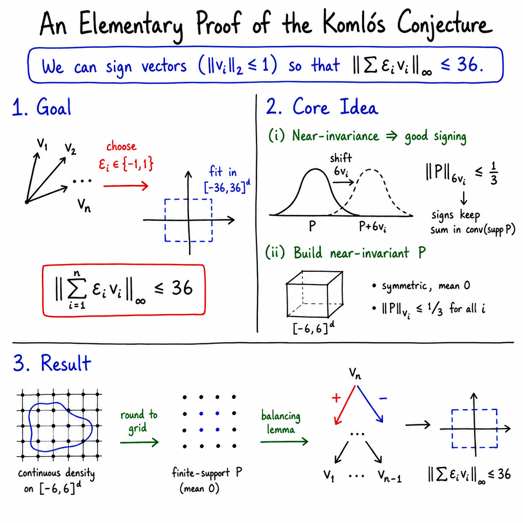
Abstract: We give an elementary proof of the Komlós conjecture by simplifying the recent proof of Guo, Fang, and Lu. We show that any vectors $v_1,\ldots,v_n\in\mathbb{R}<sup>d$ with $|v_i|<em>2\le1$ admit signs $\varepsilon_i\in{-1,1}$ such that $$|\sum</em>{i=1}^{n\varepsilon_i} v_i|_\infty\le36$$. The proof uses only elementary combinatorial and probabilistic arguments and basic calculus.

• The paper proves the Komłos conjecture with a straightforward approach, using combatorical methods, to establish that the l-infinity norm of a signed sum of vectors is bounded by 36.
• A finite-dimensional induction technique converts the near-equal distribution of points to signs ensuring the resulting vector remains near the original convex hull, which allows for an inductive process.
• A nearly translation-invariant distribution ensures the total vector variation under unit radius translations remains small, leading to a finite distribution that serves as the result of the conjecture.

Main result and context

The paper proves the Komlós conjecture with an explicit universal constant. For vectors $v_1,\ldots,v_n\in\mathbb{R}^d$ satisfying $\|v_i\|_2\le 1$, it establishes the existence of signs $\varepsilon_i\in\{-1,1\}$ such that

$$\left\|\sum_{i=1}^n \varepsilon_i v_i\right\|_\infty\le 36.$$

This resolves the conjecture in its standard, non-prefix form. The argument is deliberately nonoptimal in its constant: the paper gives $36$, whereas the contemporaneous proof of Guo, Fang, and Lu gives $3\sqrt{2\pi}$ (Guo et al., 10 Sep 2026). The contribution is instead a substantial simplification of the proof architecture. It replaces the latter paper’s use of Banaszczyk’s convex-body transform and directional total-variation analysis with finite-support combinatorics, elementary probability, and a short analytic estimate.

The Komlós conjecture asks for a dimension- and cardinality-independent bound on the $\ell_\infty$ norm of a signed sum of Euclidean unit vectors. Its significance derives partly from its relationship to discrepancy theory: it contains the Beck–Fiala conjecture as a special case and would improve substantially on the general $O(\sqrt{\log n})$ bound supplied by Banaszczyk’s vector-balancing theorem. The paper places its result after a sequence of recent improvements from $O(\sqrt{\log n})$ to $O((\log n)^{1/4})$, but its theorem is qualitatively stronger because the bound is an absolute constant.

The proof is organized around a distribution that is nearly invariant under translations by the input vectors. The central quantity is the statistical, or total variation, distance between a finitely supported distribution $\|v_i\|_2\le 1$0 and its translate $\|v_i\|_2\le 1$1:

$\|v_i\|_2\le 1$2

Small shift distance means that $\|v_i\|_2\le 1$3 and $\|v_i\|_2\le 1$4 have substantial overlapping mass. The paper exploits this overlap to convert approximate translation invariance into an exact signed balancing statement.

The balancing lemma

The first main component is a finite-dimensional induction that converts near invariance into signs. Suppose that $\|v_i\|_2\le 1$5 is a finitely supported probability distribution on $\|v_i\|_2\le 1$6 satisfying

$\|v_i\|_2\le 1$7

The paper proves that there are signs $\|v_i\|_2\le 1$8 for which

$\|v_i\|_2\le 1$9

The conclusion is stronger and more flexible than merely bounding the signed sum. It asserts that the shifted mean remains inside the convex hull of the original support. This convex-hull formulation is what permits induction: after processing one vector, the resulting convex combination can serve as the input mean for the remaining vectors.

The splitting operator

For a vector $\varepsilon_i\in\{-1,1\}$0, the proof defines a splitting operator $\varepsilon_i\in\{-1,1\}$1 that maps a distribution $\varepsilon_i\in\{-1,1\}$2 on $\varepsilon_i\in\{-1,1\}$3 to a distribution on $\varepsilon_i\in\{-1,1\}$4. A new state $\varepsilon_i\in\{-1,1\}$5 or $\varepsilon_i\in\{-1,1\}$6 has two possible parents, $\varepsilon_i\in\{-1,1\}$7 and $\varepsilon_i\in\{-1,1\}$8. The operator assigns half the larger of the two parent masses to the state with bit $\varepsilon_i\in\{-1,1\}$9 and half the smaller mass to the state with bit $$\left\|\sum_{i=1}^n \varepsilon_i v_i\right\|_\infty\le 36.$$0:

$$\left\|\sum_{i=1}^n \varepsilon_i v_i\right\|_\infty\le 36.$$1

$$\left\|\sum_{i=1}^n \varepsilon_i v_i\right\|_\infty\le 36.$$2

The operator preserves total mass and preserves the mean in the original $$\left\|\sum_{i=1}^n \varepsilon_i v_i\right\|_\infty\le 36.$$3 coordinates. The newly introduced bit coordinate has mean

$$\left\|\sum_{i=1}^n \varepsilon_i v_i\right\|_\infty\le 36.$$4

Consequently, if $$\left\|\sum_{i=1}^n \varepsilon_i v_i\right\|_\infty\le 36.$$5, then $$\left\|\sum_{i=1}^n \varepsilon_i v_i\right\|_\infty\le 36.$$6. The bit-$$\left\|\sum_{i=1}^n \varepsilon_i v_i\right\|_\infty\le 36.$$7 states therefore contain a uniformly positive amount of mass and, crucially, every such state has both possible parents available.

The operator also contracts shift distances in directions orthogonal to the new coordinate:

$$\left\|\sum_{i=1}^n \varepsilon_i v_i\right\|_\infty\le 36.$$8

where $$\left\|\sum_{i=1}^n \varepsilon_i v_i\right\|_\infty\le 36.$$9. This follows from monotonicity of the maximum and minimum operations and from the fact that the common mass of $36$0 and $36$1 is mapped to common mass of $36$2 and $36$3. Thus, adding the auxiliary bit does not degrade the near-invariance assumptions needed for the remaining vectors.

Induction and pullback

To process the final vector $36$4, the construction applies $36$5, so that the two parents differ by $36$6. The assumption $36$7 implies that the bit-$36$8 mass is at least $36$9. The induction hypothesis is then applied in one higher dimension to the lifted vectors $3\sqrt{2\pi}$0 for $3\sqrt{2\pi}$1.

The induction produces a convex combination of split states with mean

$3\sqrt{2\pi}$2

Because the last coordinate is binary, its mean $3\sqrt{2\pi}$3 specifies exactly the total mass assigned to bit-$3\sqrt{2\pi}$4 states. The proof then pulls this convex combination back to the support of $3\sqrt{2\pi}$5.

Mass on bit-$3\sqrt{2\pi}$6 states has only one available parent. Since its total mass is $3\sqrt{2\pi}$7, the resulting displacement in the $3\sqrt{2\pi}$8 direction is $3\sqrt{2\pi}$9 for some $\ell_\infty$0. Bit-$\ell_\infty$1 states have both parents available, and their total mass is at least $\ell_\infty$2. By distributing this mass between the two parents, the proof can realize any additional coefficient in an interval of length at least $\ell_\infty$3. This permits the choice of $\ell_\infty$4 so that the total displacement is exactly $\ell_\infty$5.

The numerical constants arise directly from this pullback geometry. The shift by $\ell_\infty$6 creates parent separation $\ell_\infty$7; the lower bound $\ell_\infty$8 supplies enough flexible mass; and the bound $\ell_\infty$9 ensures that one of the two signs lies within distance $O(\sqrt{\log n})$0 of $O(\sqrt{\log n})$1. The argument is elementary but carefully calibrated: the auxiliary coordinate is not merely a bookkeeping device, since its preserved mean guarantees the mass needed to correct the final signed coefficient.

Constructing a near-invariant distribution

The second main component constructs a mean-zero distribution supported in the cube $O(\sqrt{\log n})$2 whose shift distance is at most $O(\sqrt{\log n})$3 in every direction corresponding to a Euclidean unit vector.

The continuous prototype is a product density. Define the one-dimensional tent function

$O(\sqrt{\log n})$4

and let

$O(\sqrt{\log n})$5

The density $O(\sqrt{\log n})$6 is symmetric, supported on $O(\sqrt{\log n})$7, and has mean zero. The normalization and derivative identities are

$O(\sqrt{\log n})$8

The last identity eliminates mixed terms in the directional derivative calculation. For every $O(\sqrt{\log n})$9,

$O(\sqrt{\log n})$0

Applying the fundamental theorem of calculus along line segments and then Cauchy–Schwarz gives

$O(\sqrt{\log n})$1

Since $O(\sqrt{\log n})$2, another Cauchy–Schwarz estimate yields

$O(\sqrt{\log n})$3

For $O(\sqrt{\log n})$4, this is at most $O(\sqrt{\log n})$5. The implication is direct: the scale of the cube has been selected so that the density is sufficiently stable under every unit Euclidean translation, independently of the dimension.

The use of the square-root density $O(\sqrt{\log n})$6 is important. The total variation of $O(\sqrt{\log n})$7 itself is controlled indirectly through the $O(\sqrt{\log n})$8 displacement of its square root. The product structure then converts the directional energy into $O(\sqrt{\log n})$9 without dimension-dependent loss. This is the analytic core of the construction.

Discretization and completion of the proof

The balancing lemma requires finite support, whereas the preceding construction is continuous. The paper resolves this by rounding the density to a rational grid.

For rational input vectors, choose $O((\log n)^{1/4})$0 so that every $O((\log n)^{1/4})$1 has integer coordinates, and let

$O((\log n)^{1/4})$2

Round each sample from $O((\log n)^{1/4})$3 coordinatewise to the nearest point of $O((\log n)^{1/4})$4. Because the cube endpoints $O((\log n)^{1/4})$5 lie on the grid, the resulting distribution $O((\log n)^{1/4})$6 remains supported in $O((\log n)^{1/4})$7. Symmetry is preserved, so $O((\log n)^{1/4})$8.

Rounding does not increase total variation under grid translations. More precisely, if $O((\log n)^{1/4})$9, then the cell structure is compatible with translation by $\|v_i\|_2\le 1$00, and the triangle inequality gives

$\|v_i\|_2\le 1$01

Thus, for every rational input vector with norm at most $\|v_i\|_2\le 1$02,

$\|v_i\|_2\le 1$03

Applying the balancing lemma to the scaled vectors $\|v_i\|_2\le 1$04 gives signs satisfying

$\|v_i\|_2\le 1$05

Since the support lies in $\|v_i\|_2\le 1$06, the left-hand side lies in the same cube, and therefore

$\|v_i\|_2\le 1$07

The extension from rational to real vectors uses coordinatewise rational approximation within the Euclidean unit ball. Because there are finitely many sign vectors, one sign vector occurs along an infinite subsequence of approximations. Passing to the limit preserves the $\|v_i\|_2\le 1$08 bound. This compactness argument establishes the theorem for arbitrary real inputs.

The resulting proof is finite for rational data, but the paper explicitly does not claim a polynomial-time algorithm. Constructing and manipulating the discretized distribution may require support sizes and numerical representations that are not controlled polynomially in the natural input parameters. Thus, the theorem is existential and constructive in a weak finite sense, not an efficient algorithmic result.

Relation to existing proofs

The proof is a combinatorial reformulation of the mechanism underlying the proof of Guo, Fang, and Lu (Guo et al., 10 Sep 2026). That work uses an auxiliary coordinate and rearranges densities so that translation distances do not increase. Here, the rearrangement is replaced by the two-level splitting operator. The maximum/minimum assignment preserves common mass and produces a binary coordinate whose mean records the available overlap.

This replacement has two effects. It makes the proof substantially more elementary, since the essential operations are finite mass splitting, convex combinations, and total variation inequalities. It also worsens the constant, from $\|v_i\|_2\le 1$09 to $\|v_i\|_2\le 1$10. The paper does not attempt to optimize the constants, and the gap should therefore be interpreted as a consequence of proof simplification rather than as evidence of an intrinsic limitation of the method.

The result also differs fundamentally from the earlier $\|v_i\|_2\le 1$11 vector-balancing bounds and the intermediate $\|v_i\|_2\le 1$12 estimates. Those bounds retain explicit dependence on $\|v_i\|_2\le 1$13, whereas the present argument eliminates that dependence entirely. Its main technical cost is that it provides no efficient signing procedure and no prefix control.

Limitations and open questions

The theorem controls only the final signed sum. It does not establish the strong, or prefix, Komlós conjecture, which asks for a single signing satisfying

$\|v_i\|_2\le 1$14

The paper states plainly that it is unknown whether the near-invariance and splitting framework can be adapted to this setting. The obstruction is structural: the induction constructs a signing whose total displacement lies in a prescribed convex hull, but it does not maintain compatible convex-hull conditions for every prefix in the fixed input order. The same limitation applies to the proof of Guo, Fang, and Lu.

The explicit constant $\|v_i\|_2\le 1$15 is also not optimized. Several numerical choices—particularly the cube radius, the shift scale $\|v_i\|_2\le 1$16, and the threshold $\|v_i\|_2\le 1$17—are selected to make the induction transparent. It remains open within this approach how much the constant can be reduced while retaining an elementary proof.

Finally, the finite discretization establishes existence for rational inputs but does not yield a polynomial-time algorithm. The paper therefore leaves open whether this proof architecture can be made algorithmically efficient, or whether an efficient implementation would require a different representation of the near-invariant distribution.

Conclusion

The paper gives a self-contained elementary proof of the Komlós conjecture with the explicit bound

$\|v_i\|_2\le 1$18

Its central idea is to construct a mean-zero distribution in a fixed cube that is nearly invariant under all unit Euclidean translations, then use a binary splitting operator to convert this approximate invariance into exact signed balancing. The proof separates the analytic task of constructing the distribution from the combinatorial task of extracting signs, and the discretization step connects the two without dimension-dependent loss. The principal unresolved issues are constant optimization, polynomial-time constructivity, and extension from final-sum balancing to simultaneous prefix balancing.