Uncovering the Associations between Human Big Five Personality Traits and Built Environment Characteristics from Street View Imagery
Abstract: Human-environment interactions, a classic topic in geography, suggest that individuals and their environments might shape each other. Yet the specific mechanisms underlying these interactions regarding human personality traits have not been explored. This study examines the associations between human Big Five personality traits and built environment characteristics derived from street view imagery across four cities in Texas, United States, providing a descriptive foundation for understanding these complex human-environment dynamics. By integrating fine-resolution self-reported personality assessments with computer vision analysis of urban environments, we identified significant spatial clustering of personality traits at the ZIP code level. Our regression analyses reveal that built environment features and socioeconomic characteristics explain substantial variance in personality distributions, with Openness showing the strongest model fit (R2 = 0.47), followed by Agreeableness, Conscientiousness, Extraversion, and Neuroticism. Grouped built environment categories, socioeconomic factors, and demographic composition showed trait-specific patterns of association. These findings illustrate how personality traits may be associated with physical spaces at a smaller geographic scale than previously examined. Our results provide empirical evidence for understanding the link between psychological characteristics and environmental features, which can potentially enrich geography studies from a human-centered perspective.
Paper Prompts
Sign up for free to create and run prompts on this paper.
Top Community Prompts
Explain it Like I'm 14
1. What is this paper about?
This paper studies whether people’s personality traits are connected with the kinds of places where they live.
The researchers looked at four large Texas cities:
- Austin
- Dallas
- Houston
- San Antonio
They compared two types of information:
- Personality scores from more than 150,000 people.
- Images of streets and neighborhoods collected from Google Street View.
The main idea is that people and places may influence each other. For example, people who enjoy meeting others might prefer lively neighborhoods, while people who like quiet spaces might prefer areas with more open land. However, the study cannot tell whether the environment changes people’s personalities, whether people choose certain environments, or both.
2. What questions did the researchers ask?
The study focused on two main questions:
- Do personality traits form geographic patterns? In other words, are people with similar personality scores more likely to live in nearby neighborhoods?
- Are personality traits connected with features of the built environment? The built environment means the human-made parts of a place, such as buildings, roads, sidewalks, fences, cars, greenery, and open spaces.
The researchers used the Big Five personality traits:
| Trait | Simple meaning |
|---|---|
| Openness | Being curious, creative, and interested in new ideas |
| Conscientiousness | Being organized, responsible, and dependable |
| Extraversion | Being outgoing, social, and energetic |
| Agreeableness | Being kind, cooperative, and understanding |
| Neuroticism | Being more likely to experience worry, stress, or emotional ups and downs |
These traits do not label people as “good” or “bad.” They simply describe general differences in how people tend to think, feel, and behave.
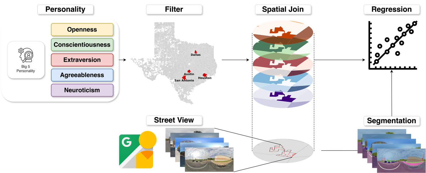
3. How did the researchers conduct the study?
Collecting personality information
The researchers used an online personality project in which people completed questionnaires about themselves. Their answers were used to calculate scores for the Big Five traits.
The researchers then grouped the participants by their ZIP codes. Instead of studying each person separately, they calculated the average personality score for each ZIP-code area. This also helped protect people’s privacy.
The final personality dataset included:
- About 150,000 participants
- 340 ZIP-code areas
- Information collected between 2010 and 2020
Studying the neighborhoods
The researchers used about five million street-view images taken across the four cities. Images were collected about every 100 meters, which is roughly the length of a city block.
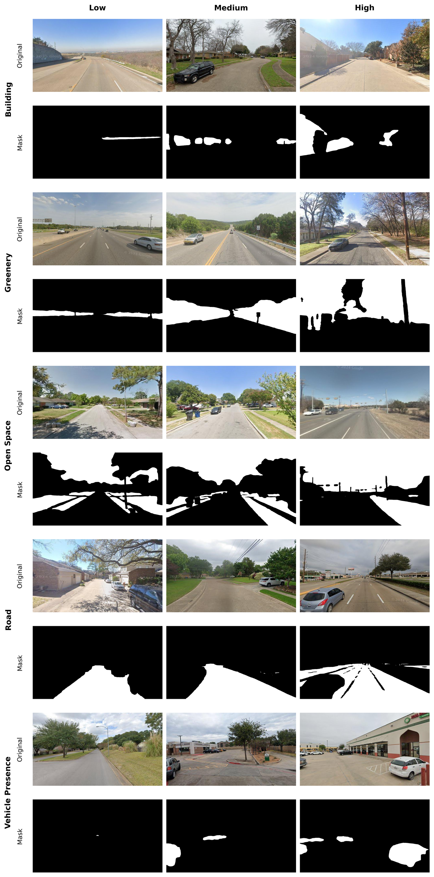
They used artificial intelligence, or AI, to examine the images. The AI used two main techniques:
- Semantic segmentation: The computer labels parts of an image pixel by pixel. For example, it can identify which pixels show buildings, roads, trees, cars, or sky. This is similar to giving every part of a photograph a colored label.
- Object detection: The computer looks for individual objects, such as cars, people, security cameras, or American flags. This is similar to asking someone to count all the bicycles or trees in a picture.
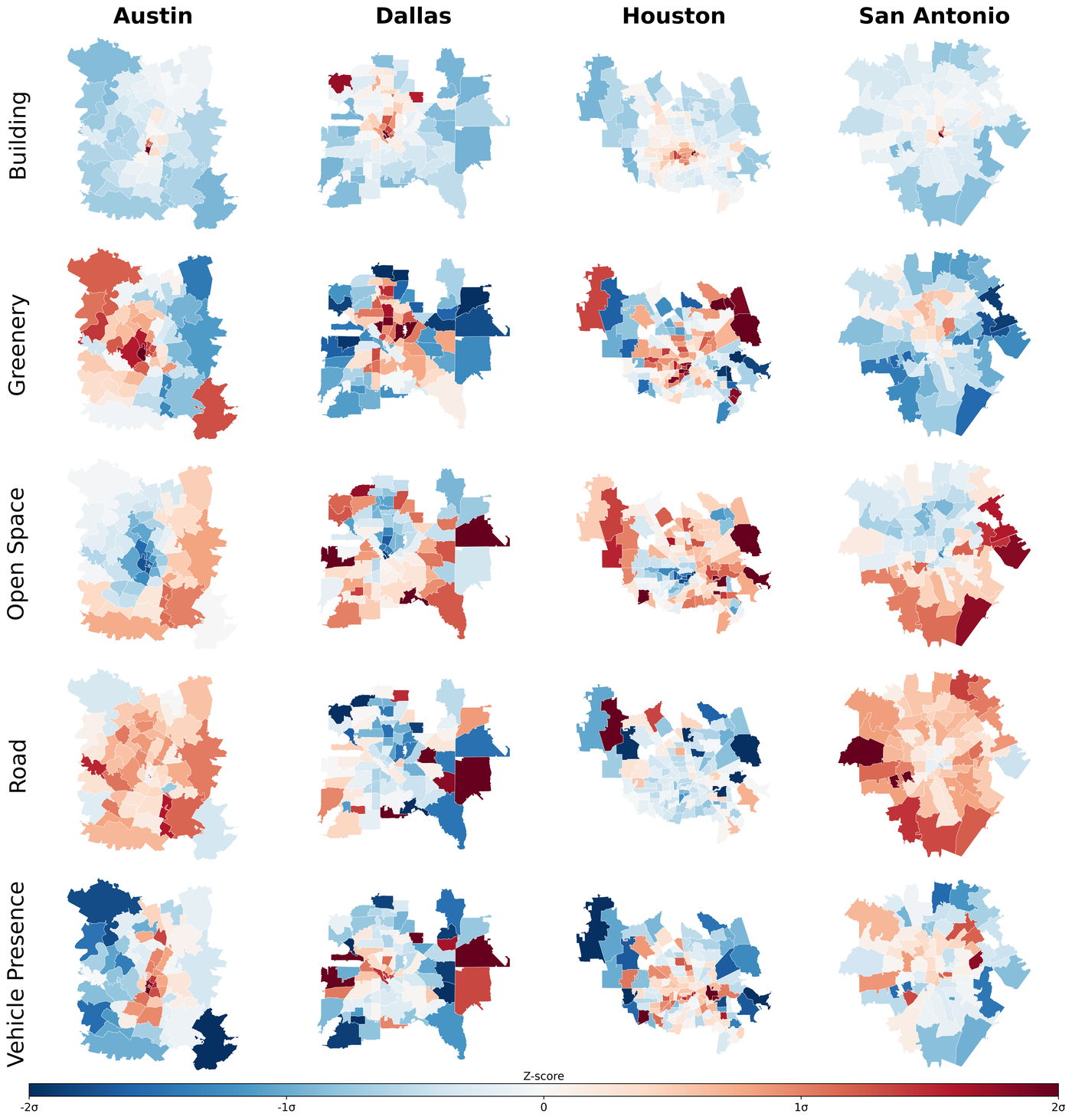
The researchers grouped these features into larger categories, including:
- Greenery
- Open space
- Buildings
- Roads
- Walking and cycling infrastructure
- Cars and other vehicles
- Physical boundaries such as fences
- People using active transportation
They also included information from the U.S. Census, such as age, income, population density, gender, and racial diversity.
Looking for patterns
The researchers used several statistical tools:
- Moran’s I: A test that checks whether nearby areas have similar values. It is like asking whether neighborhoods with high scores tend to be next to other high-score neighborhoods.
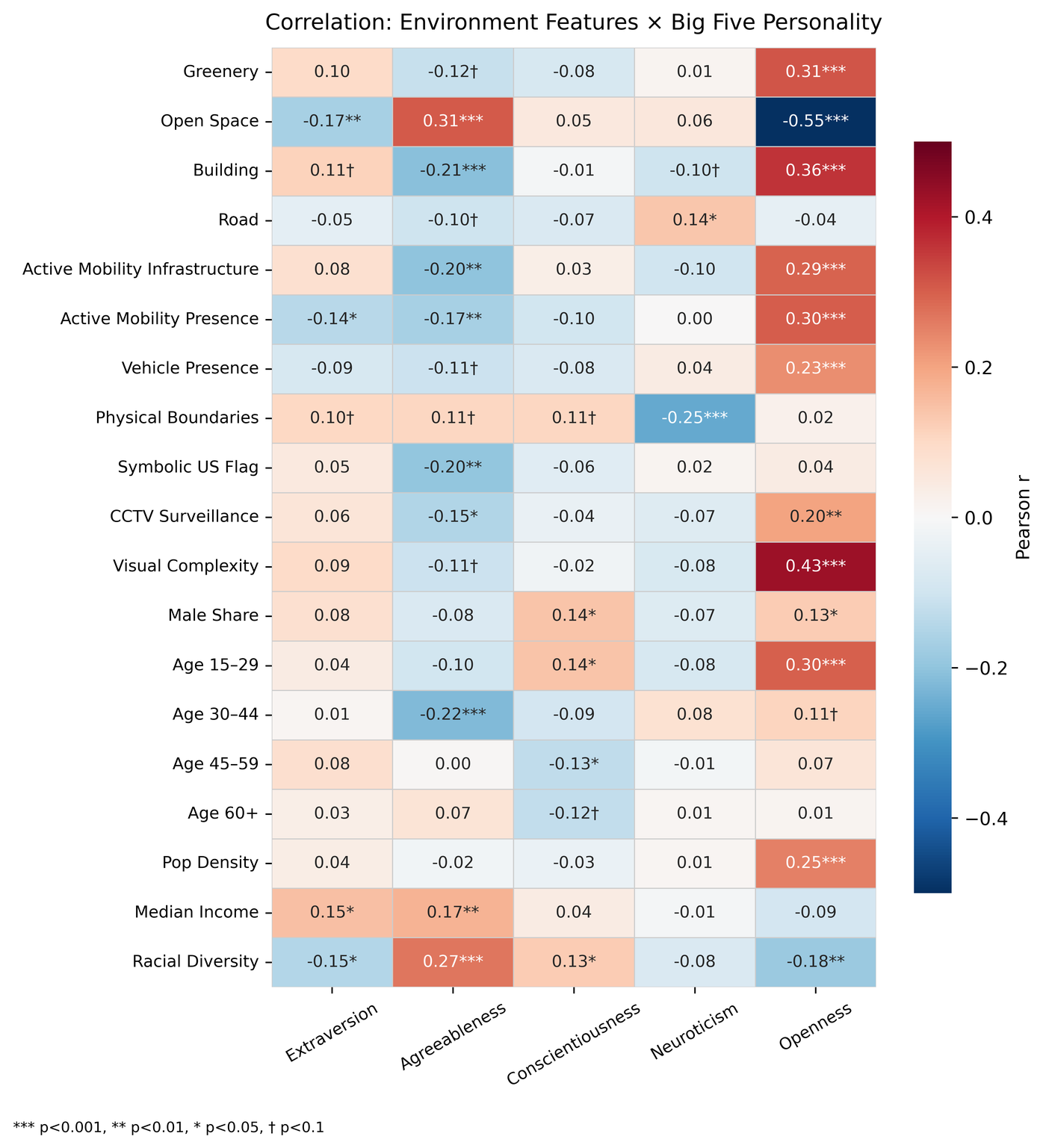
- Correlation: A measure of whether two things tend to change together. For example, it can show whether areas with more greenery also tend to have higher or lower average scores for a personality trait.
- Regression models: These are mathematical methods for estimating how several factors are related to an outcome at the same time. They are similar to trying to predict a student’s test score using several clues, such as study time, sleep, and class attendance.
- Spatial models: Because nearby neighborhoods may resemble one another, the researchers used a special model that accounts for geographic closeness.
These methods show associations, or relationships. They do not prove that one factor directly causes another.
4. What did the researchers find?
Personality traits were clustered geographically
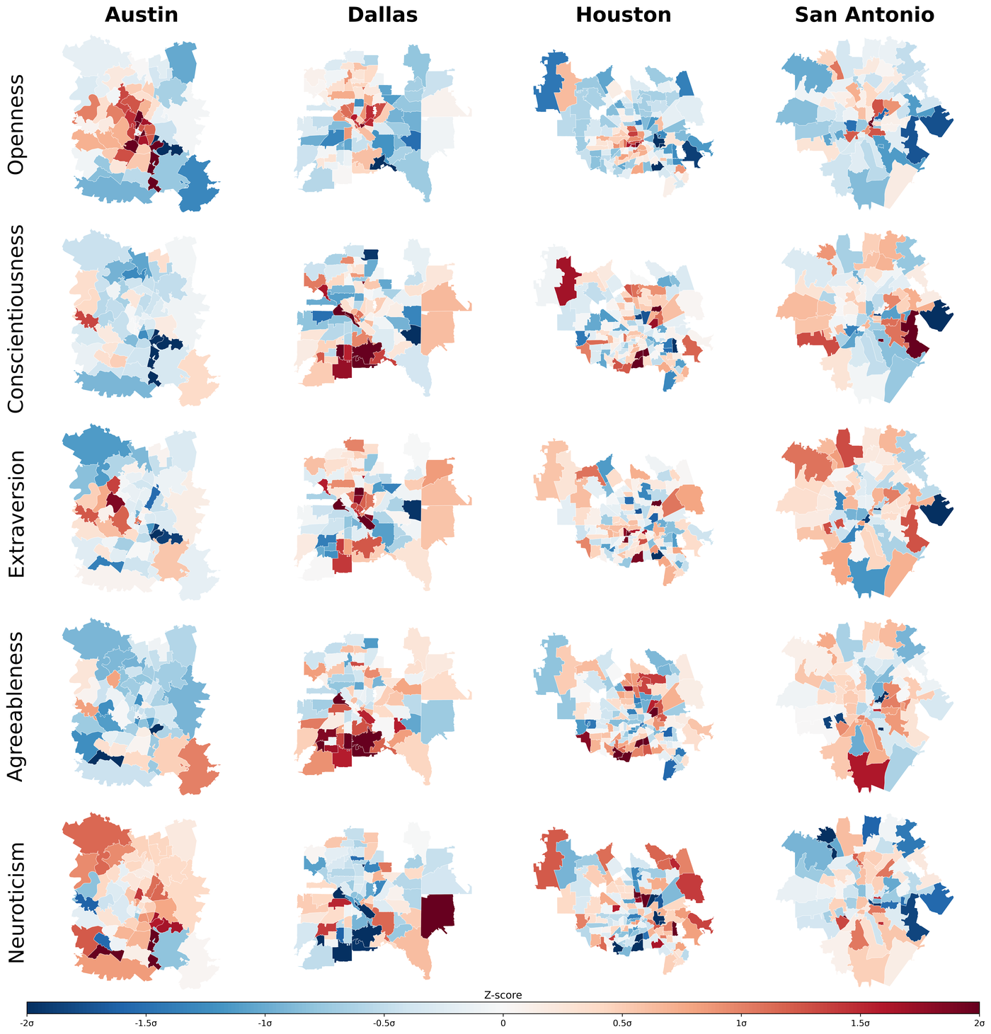
All five personality traits showed significant geographic clustering. This means that nearby ZIP-code areas often had similar average personality scores.
The strongest clustering was found for Agreeableness. The other traits also showed clustering, but less strongly.
Examples of the patterns included:
- Openness tended to be higher in central parts of Austin and lower in some outer areas.
- Conscientiousness was especially high in parts of southwestern Dallas.
- Extraversion was often higher in central Austin and Dallas.
- Agreeableness was higher in parts of southern Dallas and Houston.
- Neuroticism was relatively high across many Austin neighborhoods and lower in some parts of Dallas.
These patterns suggest that personality is not spread randomly across cities.
Different traits were associated with different environments
The relationships between personality and neighborhood features were not all the same.
Openness
Openness had the strongest overall statistical model. It was related to features such as:
- More visual complexity
- More buildings
- More greenery
- More walking and cycling activity
- Greater population density
However, the detailed regression analysis showed that age groups explained much of the variation in Openness. Physical features of the environment were not clearly significant after other factors were considered.
This is an important warning: a simple relationship between Openness and buildings or greenery may partly reflect the kinds of people living in those neighborhoods, including their ages.
Conscientiousness
Conscientiousness had several negative associations with environmental features. It tended to be lower in areas with more:
- Open space
- Greenery
- Buildings
- Roads
- Fences or other physical boundaries
- Population density
The researchers found this trait had more connections with built-environment features than the other traits. Still, these results describe neighborhood-level patterns and do not mean that living near trees or roads makes someone less conscientious.
Agreeableness
Agreeableness was generally associated with:
- More open space
- Greater racial diversity
- Higher household income
It tended to be lower in places with more buildings, some types of walking infrastructure, and physical boundaries such as fences.
Extraversion
Extraversion was associated with:
- Higher household income
- More buildings and roads in some analyses
It was negatively related to open space, active mobility presence, and racial diversity in the correlation analysis.
Neuroticism
Neuroticism showed fewer strong relationships with the built environment. It was associated with:
- More roads
- Fewer physical boundaries
The model explained less of the differences in Neuroticism than it did for Openness or Agreeableness.
How well could the models explain personality differences?
The researchers used a number called . This number tells us how much of the differences between neighborhoods the model could explain. A higher number means the model explained more, but it does not mean the model proved causation.
The results were approximately:
| Personality trait | Amount explained by the model |
|---|---|
| Openness | 47% |
| Agreeableness | 35% |
| Conscientiousness | 21% |
| Extraversion | 18% |
| Neuroticism | 16% |
The model explained Openness best, although much of that explanation came from demographic information, especially the ages of residents.
5. Why are these findings important?
This research is important because it examines personality at a smaller neighborhood scale than many earlier studies. Previous research often compared countries, states, or large regions. This paper looked at places where people experience their surroundings every day.
The study also shows how street-view images and AI can help researchers study cities. Instead of sending people to inspect every street, computers can examine millions of images and measure features consistently.
However, the results should be interpreted carefully:
- The study found relationships, not definite causes.
- It cannot show whether places shape personality or whether people with certain personalities choose particular places.
- The personality data were self-reported.
- The street-view images and personality information were collected during different years.
- ZIP-code averages do not describe every individual who lives in an area.
- Some ZIP codes had to be removed because they did not have enough participants or image coverage.
Conclusion: What could this research lead to?
The paper suggests that personality and the built environment may be connected in complicated ways. People may choose neighborhoods that fit their preferences, and living in a certain kind of place may also influence their experiences over time.
In the future, this type of research could help urban planners understand how different people experience neighborhoods. It might support the design of places that offer a healthy mix of greenery, open space, safe streets, buildings, transportation options, and opportunities for social interaction.
The research does not mean that a neighborhood determines someone’s personality. Instead, it provides an early map of possible connections between people’s psychological characteristics and the physical spaces around them. Further studies would need to follow people over time to discover how these relationships actually develop.
Knowledge Gaps
The paper leaves the following knowledge gaps, limitations, and open questions unresolved:
- Causal direction remains unidentified: The cross-sectional, observational design cannot determine whether built environments influence personality, whether people with particular traits select into certain neighborhoods, or whether both processes operate simultaneously.
- Selective migration is not directly measured: The study does not include residential histories, migration flows, duration of residence, housing choices, or reasons for moving, leaving the role of personality-based sorting unresolved.
- Environmental influence over the life course is untested: There is no evidence on whether exposure to specific built-environment features during childhood, adolescence, or adulthood predicts later personality development.
- Bidirectional feedback mechanisms are not empirically modeled: Although the paper theorizes that residents may shape their environments and environments may shape residents, it does not measure resident preferences, civic participation, investment, or neighborhood change.
- Individual-level mechanisms are obscured by ZCTA aggregation: Associations between average personality scores and average neighborhood characteristics cannot establish that individuals exposed to particular features possess the corresponding traits; ecological fallacy remains a major concern.
- Within-neighborhood heterogeneity is not examined: ZCTAs may contain substantial variation in housing types, street design, land use, socioeconomic conditions, and personality composition that is masked by averaging.
- The appropriate spatial scale is unresolved: The analysis does not test whether associations differ at street, block, tract, neighborhood, or city scales, nor whether results are sensitive to the modifiable areal unit problem.
- Residential exposure is approximated rather than observed: Participants are assigned environmental characteristics based on ZIP-code residence, but the study does not account for daily activity spaces, workplaces, schools, commuting routes, or time spent outside the home neighborhood.
- Personality sample representativeness is uncertain: Participants in the Gosling–Potter Internet Project are self-selected online respondents and may differ from the broader Texas population in age, education, internet access, socioeconomic status, motivation, and cultural background.
- Geographic selection into the dataset may bias results: The number of participants varies substantially across ZCTAs, and areas with few or no respondents may systematically differ from areas with high participation.
- The participant filtering criteria require clarification and validation: The table reports a minimum of three participants per ZIP code, whereas the methods state that ZCTAs with fewer than 20 participants were excluded. The implications of this discrepancy for reliability and reproducibility are unresolved.
- Reliability of ZCTA-level personality means is not fully quantified: The paper does not report confidence intervals, intraclass reliability, shrinkage estimates, or sensitivity analyses showing how trait means change with different minimum sample-size thresholds.
- Measurement equivalence across assessment instruments is assumed: BFI and BFI-2 responses are pooled, but the study does not demonstrate that scores are comparable across versions, collection years, demographic groups, or language contexts in this specific sample.
- Self-report and response biases are not addressed: Acquiescence, social desirability, careless responding, and differences in scale use could contribute to spatial variation in mean personality scores.
- Temporal mismatch between personality and imagery remains consequential: Personality data span 2010–2020, while SVI imagery spans 2007–2025. Aggregating across these periods may pair personality measurements with environments that did not exist at the time of assessment, especially in rapidly changing neighborhoods.
- Historical imagery is not modeled as a time-varying exposure: The study uses available imagery to maximize coverage but does not determine which image date best represents participants’ environments or analyze environmental change over time.
- Street View coverage may be systematically incomplete: Areas with sparse imagery, restricted access, private roads, poor image quality, or limited historical coverage may be excluded or underrepresented, potentially biasing environmental measures.
- SVI captures only visually observable conditions: Important environmental attributes—noise, air quality, thermal comfort, odors, accessibility, maintenance quality, indoor conditions, social interactions, and perceived safety—are not directly measured.
- Computer-vision measurement validity is insufficiently established for this context: The accuracy of Mask2Former and GroundingDINO classifications is not reported separately for the four Texas cities, different urban forms, weather conditions, camera perspectives, or image dates.
- Object-detection errors may affect count-based predictors: False positives and false negatives for pedestrians, vehicles, flags, CCTV cameras, and other objects are not quantified or propagated into the regression uncertainty.
- Image-derived features may reflect camera and sampling artifacts: Differences in image heading, panorama selection, season, lighting, weather, camera generation, and grid-point placement may influence measured greenery, sky, road, and visual-complexity values.
- The composite environmental categories lack sensitivity analysis: Summing heterogeneous features into categories such as “Greenery,” “Road,” or “Physical Boundaries” assumes equal substantive importance and compatible measurement properties, but alternative weighting schemes or dimensionality-reduction methods are not tested.
- The construct validity of symbolic and surveillance indicators is unclear: Counts of American flags and detected CCTV cameras may be weak or context-dependent proxies for political identity, neighborhood control, perceived safety, or social climate.
- Visual complexity is not linked to perceptual validation: The segmentation-based complexity measure is not compared with human ratings or alternative measures of streetscape complexity.
- Important built-environment dimensions are omitted: The analysis does not directly measure building height, architectural style, façade condition, land-use mix, sidewalk continuity, intersection density, transit access, noise, accessibility, housing tenure, or public-space quality.
- Socioeconomic and demographic controls are incomplete: Potential confounders such as education, employment, poverty, housing costs, tenure, immigration status, household structure, crime, health, political context, and historical segregation are not included.
- Residual confounding may explain the reported associations: Demographic composition and built-environment variables are strongly spatially patterned, making it difficult to determine whether estimated coefficients reflect physical features, neighborhood socioeconomic status, or broader urban structure.
- Multicollinearity treatment may introduce specification bias: Iteratively removing predictors according to VIF and retaining only variables with significant bivariate correlations can eliminate theoretically important confounders and produce unstable coefficient estimates.
- Bivariate preselection creates risks of data-driven inference: Selecting variables based on their observed correlations with the outcomes may induce selection bias, inflate apparent significance, and make the reported models difficult to replicate in new samples.
- Multiple hypothesis testing is not fully controlled: Numerous traits, environmental variables, controls, transformations, and model specifications are examined, but no correction for multiple comparisons or preregistered hypothesis set is reported.
- Spatial dependence is handled incompletely: The paper uses Moran’s I and spatial lag models, but does not compare alternative spatial error, spatial Durbin, geographically weighted, multilevel, or spatially varying-coefficient models.
- The spatial-weight specification is not tested for robustness: Results may depend on Queen contiguity, especially for irregular or disconnected ZCTAs, yet alternative distance-based or k-nearest-neighbor matrices are not evaluated.
- Spatial lag interpretation is potentially ambiguous: A spatial lag of neighborhood personality may reflect diffusion, shared omitted causes, migration, or measurement smoothing; the study does not distinguish among these explanations.
- Model assumptions are not comprehensively assessed: Evidence is not provided regarding heteroskedasticity beyond the use of HC1 errors, nonlinearity, influential ZCTAs, residual spatial autocorrelation, normality, or functional-form sensitivity.
- Cross-city comparability is uncertain: City fixed effects absorb average differences but do not test whether associations vary by city, urban form, race, climate, or local institutional context through interaction terms or hierarchical models.
- Generalizability beyond large Texas cities is unknown: Findings may not transfer to other U.S. regions, smaller cities, rural areas, older cities, suburbs outside Texas, or non-U.S. cultural and planning contexts.
- Neighborhood personality distributions may be influenced by institutional composition: Universities, military bases, prisons, assisted-living facilities, and other institutions could alter both participant composition and environmental appearance, but are not explicitly considered.
- The practical implications are not evaluated: The study does not establish whether modifying greenery, open space, roads, surveillance, or other features would change personality-related outcomes or improve well-being.
- Potential stigmatization and privacy risks are unexplored: Mapping personality traits at neighborhood scale could reinforce stereotypes, affect housing or investment decisions, or create privacy harms, yet ethical safeguards and responsible-use criteria are not developed.
- Replication and out-of-sample validation are absent: The models are evaluated within the same set of 255 ZCTAs used for estimation; predictive performance on held-out neighborhoods, cities, time periods, or independent personality datasets is not demonstrated.
- The incomplete reporting of the statistical results limits interpretation: The supplied results section ends during the discussion of the regression findings, leaving unresolved the full spatial-model results, coefficient differences between OLS and SLM, robustness checks, and final interpretation of significant associations.
Practical Applications
Immediate Applications
The study provides a deployable workflow—aggregating Big Five survey data by neighborhood, extracting built-environment indicators from street-view imagery, and modeling spatial associations—that can already support descriptive planning and research applications. Because the findings are correlational and based on four Texas cities, these applications should be used for diagnosis and prioritization rather than individual prediction or causal intervention.
- Urban planning and neighborhood diagnostics: Municipal planning departments can use
ZenSVI-style image segmentation and object detection to create neighborhood dashboards covering greenery, open space, buildings, roads, active-mobility infrastructure, vehicles, physical boundaries, visual complexity, and surveillance equipment. These layers can be compared with aggregated psychological and demographic indicators to identify areas warranting further planning attention.- Sector: Urban planning, GIS, placemaking.
- Potential workflow: Download or license street-view imagery → run semantic segmentation and object detection → aggregate indicators to census units → combine with ACS and survey data → map spatial clusters and model associations.
- Dependencies: Current imagery coverage, image licensing, model accuracy, sufficient neighborhood-level survey samples, and local validation.
- Human-centered placemaking: Designers can incorporate the study’s trait-specific associations into exploratory alternatives for public-space design. For example, areas associated with higher Conscientiousness were negatively related to greenery, open space, buildings, roads, and physical boundaries in the reported model, while Agreeableness was associated with open space, racial diversity, income, and lower levels of physical boundaries. These results can motivate comparison of alternative streetscape designs rather than justify a single “personality-optimized” design.
- Sector: Architecture, landscape architecture, public-space design.
- Potential products: Scenario-planning tools that compare tree cover, permeability, fencing, building density, and pedestrian infrastructure.
- Dependencies: The associations must not be interpreted as evidence that changing a physical feature will change personality; resident preferences and accessibility must be assessed directly.
- Prioritization of walkability and public-field audits: Transportation and public-health agencies can use the active-mobility and road indicators to prioritize field audits of sidewalks, crossings, bicycle facilities, pedestrian activity, and vehicle dominance. The study found that several personality patterns were associated with mobility-related features, although the direction and strength varied by trait.
- Sector: Transportation, public health, active mobility.
- Potential workflow: Use SVI-derived indicators to screen neighborhoods → conduct on-site validation → collect pedestrian counts and resident perceptions → prioritize low-cost safety or accessibility improvements.
- Dependencies: Visual presence does not necessarily measure infrastructure quality, usability, accessibility, or actual travel behavior.
- Environmental-equity screening: Analysts can overlay built-environment measures with income, age composition, racial diversity, and neighborhood-level psychological indicators to identify uneven distributions of amenities or environmental burdens. The positive association between Agreeableness and racial diversity and income, and the negative association between Extraversion and racial diversity in the pooled model, illustrate how psychological patterns may be examined alongside—not substituted for—equity indicators.
- Sector: Public policy, environmental justice, community development.
- Potential outputs: Equity maps, capital-improvement prioritization lists, and community-engagement plans.
- Dependencies: Avoiding ecological stereotyping, protecting small-area privacy, and involving affected communities in interpreting results.
- Academic training and reproducible GeoAI research: Universities can use the paper’s pipeline as a teaching and research template for combining psychological survey data, census geography, computer vision, spatial autocorrelation, OLS, and spatial lag models.
- Sector: Geography, psychology, urban studies, data science.
- Potential tools: Reproducible Python notebooks using GIS libraries,
ZenSVI, segmentation models such as Mask2Former, object detection models such as GroundingDINO, Moran’s I diagnostics, and spatial regression packages. - Dependencies: Reproducible access to imagery and survey data, documentation of model versions, and careful treatment of spatial scale and missing data.
- Neighborhood-level well-being research: Public-health and social-science researchers can use the approach to generate hypotheses about how visual environments relate to psychological well-being, social interaction, or perceived safety. The models can identify candidate locations for direct surveys, interviews, or behavioral observation.
- Sector: Public health, environmental psychology, community research.
- Dependencies: Direct individual-level measures are needed to connect environments with outcomes; aggregated personality scores cannot establish individual psychological effects.
- Improved urban-data inventories: Local governments and infrastructure companies can use automated SVI analysis to update inventories of buildings, vegetation, road markings, vehicles, fences, pedestrians, flags, and CCTV cameras more frequently than traditional manual surveys.
- Sector: Smart cities, asset management, municipal operations.
- Potential products: Change-detection systems, street-condition portals, and planning-support dashboards.
- Dependencies: Temporal consistency of imagery, detection bias across neighborhoods, weather and lighting conditions, and human review of automated outputs.
Long-Term Applications
The following applications would require longitudinal data, broader geographic validation, causal designs, stronger privacy protections, or substantial technical development. The current paper should not be used to infer that built environments cause specific personality traits or to predict an individual’s personality from their location or appearance.
- Causal evaluation of psychologically supportive urban design: Future studies could test whether changes such as adding greenery, opening public space, reducing hostile physical boundaries, or improving pedestrian infrastructure affect stress, social connection, activity, or self-reported well-being over time.
- Sector: Urban policy, public health, environmental psychology.
- Required development: Quasi-experimental or experimental designs, baseline and follow-up surveys, comparison neighborhoods, and individual-level exposure histories.
- Key assumption: Environmental influence can be separated from selective migration, socioeconomic change, and pre-existing neighborhood differences.
- Longitudinal person–place interaction models: Linking repeated personality assessments, residential histories, migration records, and time-stamped SVI could distinguish selective migration from environmental influence. A neighborhood-by-year panel could examine whether personality distributions change after major redevelopment.
- Sector: Population geography, psychology, urban economics.
- Potential methods: Panel spatial models, individual fixed effects, natural experiments, and mobility trajectories.
- Dependencies: Consent-based linkage, adequate sample sizes per time period, consistent imagery, and reliable residential histories.
- Urban-design recommendation systems: A future planning platform could estimate how proposed changes to street form might affect perceived safety, sociability, walkability, or other psychosocial outcomes for different resident groups.
- Sector: Architecture, urban simulation, civic technology.
- Potential products: GIS-based “what-if” design tools, generative streetscape simulators, and multi-objective planning systems.
- Dependencies: Causal evidence, resident preference data, validated visual simulations, and safeguards against designing neighborhoods for assumed personality types.
- Personalized location and housing services: Real-estate or relocation platforms might eventually offer environment-preference matching based on a user’s stated preferences for density, greenery, open space, visual complexity, and mobility infrastructure. Such systems should match explicit preferences—not infer personality from ZIP code.
- Sector: Real estate, mobility, consumer software.
- Dependencies: User consent, anti-discrimination compliance, avoidance of protected-class proxies, and evidence that environmental preferences generalize beyond the Texas sample.
- Population-level mental-health and resilience planning: If future research establishes reliable links between environmental exposures and mental-health outcomes, cities could use SVI and spatial models to identify neighborhoods for cooling, greening, noise reduction, social-space improvements, or service delivery.
- Sector: Healthcare, public health, emergency and resilience policy.
- Dependencies: Clinical or validated well-being outcomes, environmental exposure measurements, medical privacy protections, and causal validation. Personality scores alone are not suitable for diagnosis or risk prediction.
- Cross-city and cross-cultural urban benchmarking: Applying the same computer-vision pipeline to cities outside Texas could reveal which associations are robust and which depend on local culture, climate, governance, housing markets, or transportation systems.
- Sector: Comparative urban research, international development, policy evaluation.
- Potential outputs: Harmonized urban-environment indicators and cross-city planning benchmarks.
- Dependencies: Comparable street-view coverage, culturally valid personality instruments, domain adaptation for computer-vision models, and consistent spatial units.
- Fairness-aware urban AI systems: Future systems could audit whether automated imagery analysis systematically performs worse in low-income, minority, suburban, or poorly photographed areas. This would support responsible use of GeoAI in public investment and policy.
- Sector: AI governance, civic technology, public administration.
- Potential tools: Model-audit dashboards, uncertainty maps, human-in-the-loop review, and bias-adjusted spatial estimates.
- Dependencies: Representative validation data, transparent model documentation, and governance rules preventing neighborhood labels from becoming stigmatizing classifications.
- Privacy-preserving neighborhood analytics: Because personality is sensitive psychological information, future applications could use differential privacy, minimum-cell-size rules, secure data enclaves, or federated analysis to produce neighborhood insights without exposing individual respondents.
- Sector: Data governance, academia, government.
- Dependencies: Formal privacy guarantees, legal review, informed consent, and careful disclosure-control evaluation.
- Integrated digital twins of human-centered cities: At larger scale, validated relationships between urban form, perception, behavior, and well-being could be incorporated into urban digital twins for testing redevelopment, transportation, and resilience scenarios.
- Sector: Smart cities, robotics, urban simulation, infrastructure planning.
- Dependencies: Much richer multimodal data—including mobility, health, perception, and longitudinal behavioral data—alongside causal models rather than cross-sectional correlations.
- Policy design based on heterogeneity rather than neighborhood labeling: The most defensible long-term policy use is to identify diverse resident preferences and test inclusive design options. A policy system could evaluate whether an intervention benefits residents with different ages, socioeconomic circumstances, mobility needs, and psychological preferences.
- Sector: Public policy, participatory planning.
- Dependencies: Direct community participation, representative sampling, transparent uncertainty reporting, and strict prohibition on using neighborhood personality averages to allocate rights, services, credit, housing access, policing, or employment opportunities.
Glossary
- Adjusted : A version of the coefficient of determination adjusted for the number of predictors in a regression model. “adjusted = 0.416”
- Active mobility infrastructure: Physical infrastructure supporting walking and cycling, such as sidewalks and bicycle lanes. “Active Mobility Infrastructure”
- Active mobility presence: The observed presence of people engaged in walking or cycling within the environment. “Active Mobility Presence”
- Administrative boundary: A legally or institutionally defined geographic division used for spatial analysis. “Most studies have used administrative boundaries (countries, states, counties) as the geographic unit of analysis”
- American Community Survey (ACS): A U.S. Census Bureau survey providing regularly updated demographic and socioeconomic data. “The socio-demographic and socioeconomic variables were derived from the U.S. Census Bureau’s American Community Survey (ACS) 2020 5-Year Estimates”
- Bivariate correlation: A statistical measure describing the association between two variables. “Our variable selection process was based on bivariate correlation tests between built environment elements and personality traits.”
- Big Five Inventory (BFI): A standardized psychological questionnaire measuring the five major personality dimensions. “The platform employs the Big Five Inventory (BFI) and its successor the Big Five Inventory-2 (BFI-2)”
- Bidirectional feedback loop: A process in which two related systems each influence the other over time. “These processes likely operate bidirectionally, creating feedback loops where personality and place mutually shape each other”
- Biome: A large ecological region characterized by particular climate conditions and biological communities. “These cities represent the four largest urban centers in Texas, providing a comparable regional context in terms of governance structure, climate, biome”
- Box–Cox transformation: A power transformation used to reduce skewness and make a variable’s distribution more nearly normal. “For environmental variables with significant skewness, we applied Box-Cox transformations to approximate normal distributions”
- Built environment: Human-made physical surroundings, including buildings, roads, infrastructure, and open spaces. “The built environment serves as the setting for most daily human experiences.”
- City-fixed effects: Model terms that control for unobserved characteristics shared by observations within the same city. “These binary variables function as city-fixed effects.”
- Coefficient of determination (): The proportion of variation in a dependent variable explained by a regression model. “with the highest observed for Openness ( = 0.467”
- Composite score: A single measure formed by combining multiple related variables. “For each category, we created composite scores by summing constituent variables”
- Computer vision: Artificial-intelligence methods that enable computers to interpret and analyze images or video. “When combined with computer vision and machine learning techniques, this imagery enables researchers to quantify various elements of the urban landscape.”
- Confounding: Distortion of an estimated relationship caused by an additional variable associated with both the explanatory and outcome variables. “to address confounding from neighborhood composition”
- Conscientiousness: A personality trait associated with organization, responsibility, and dependability. “Conscientiousness: The degree of organization, responsibility, and dependability.”
- Contiguity: A spatial relationship in which geographic units are treated as neighbors because they share a boundary or vertex. “defined by a spatial-weights matrix constructed using Queen contiguity”
- Demographic composition: The distribution of population characteristics such as age, sex, and race within an area. “the spatial variation in Openness is more closely linked to neighborhood demographic composition”
- Ecological influence: The process by which characteristics of a broader social or geographic context are associated with individual or group psychological characteristics. “Theoretical frameworks explain geographic variation in psychological traits through mechanisms like selective migration, environmental influence, social influence, and ecological influence”
- Environmental influence: The process through which physical surroundings affect psychological development or behavior. “environmental influence, where built characteristics shape personality development through direct exposure and social interactions”
- Extraversion: A personality trait associated with sociability, assertiveness, and positive emotionality. “Extraversion: The degree of sociability, assertiveness, and positive emotionality.”
- Fine-grained analysis: Analysis conducted using highly detailed variables or small geographic units. “This underscores the potential value of examining the associations between personality distributions and built environment characteristics at the fine-grain resolution”
- Geographic psychology: An interdisciplinary field examining how psychological characteristics vary across geographic locations and relate to place. “Study advances geographic psychology through GeoAI approaches and fine-scale analysis”
- Geospatial artificial intelligence (GeoAI): The application of artificial-intelligence methods to geospatial data and geographic problems. “the analysis of built environments using SVI and geospatial artificial intelligence (GeoAI)”
- Geographic aggregation: The process of combining individual observations into geographic units for analysis. “allowing for geographic aggregation and analysis”
- Greenery: Vegetation and plant cover visible within an urban environment. “To improve model interpretability and reduce the number of predictors, we grouped the fine-grained segmentation and detection variables”
- HC1 robust standard error: A heteroskedasticity-consistent estimate of regression uncertainty using a finite-sample correction. “OLS standardized coefficients () for Big Five personality traits and environmental predictors (pooled model, HC1 robust SE).”
- Heterogeneity: Variation in characteristics or relationships across geographic areas or groups. “to absorb city-level unobserved heterogeneity”
- Image segmentation: The division of an image into regions or pixels assigned to meaningful semantic categories. “(2) data processing (spatial join, image segmentation)”
- Intra-city variation: Differences occurring among neighborhoods or areas within the same city. “The visualized personality distributions exhibit intra-city variation”
- Machine learning: Computational methods that learn patterns from data to make predictions or classifications. “When combined with computer vision and machine learning techniques”
- Mask2Former: A deep-learning model for image segmentation that predicts masks and semantic categories. “We used the Mask2Former model pre-trained on the Mapillary Vistas dataset”
- Median household income: The income value dividing households into two equal-sized groups within a geographic area. “median household income”
- Moran’s I: A statistic measuring spatial autocorrelation, or similarity among geographically neighboring observations. “We conducted Moran's I tests”
- Neuroticism: A personality trait associated with emotional instability, anxiety, and negative emotionality. “Neuroticism: The degree of emotional instability, anxiety, and negative emotionality.”
- Object detection: A computer-vision task that identifies and locates individual objects in images. “Object Detection: This approach identifies specific objects within images”
- Ordinary Least Squares (OLS): A regression method that estimates coefficients by minimizing the squared prediction errors. “Following confirmation of spatial patterns, we developed Ordinary Least Squares (OLS) regression models”
- Openness: A personality trait associated with intellectual curiosity, creativity, and preference for novelty. “Openness: The degree of intellectual curiosity, creativity, and preference for novelty.”
- Pearson correlation coefficient: A statistic measuring the strength and direction of a linear relationship between two variables. “The correlation analysis revealed distinct patterns across personality traits.”
- Physical boundaries: Structures such as fences or walls that visually or physically separate spaces. “Physical Boundaries”
- Place identity: The meanings and characteristics through which a location becomes associated with individual or collective identity. “These unique place characteristics contribute to the formation of place identities”
- Population density: The number of people living within a specified unit of land area. “population density”
- Queen contiguity: A spatial-neighbor definition in which two areas are neighbors if they share either an edge or a vertex. “Under this specification, two ZCTAs are considered neighbors if they share a boundary or vertex”
- Racial diversity index: A quantitative measure representing the variety and relative distribution of racial groups in a population. “a racial diversity index”
- Selective migration: The movement of people toward or away from locations based on their characteristics or preferences. “selective migration, where individuals choose locations aligned with their traits”
- Semantic segmentation: Pixel-level classification of an image into predefined semantic categories. “This technique classifies each pixel in an image into predefined categories”
- Spatial adjacency: The geographic relationship between areas that share a boundary or vertex. “which captures the spatial adjacency structure of the study area.”
- Spatial autocorrelation: The degree to which nearby geographic observations have similar or dissimilar values. “These results indicate that similar personality trait levels tend to cluster in geographically proximate areas”
- Spatial dependence: A condition in which observations are statistically related because of their geographic proximity. “To account for this spatial dependence, we estimated the Spatial Lag Model (SLM)”
- Spatial Lag Model (SLM): A regression model that includes neighboring observations of the dependent variable to account for spatial dependence. “To account for this spatial dependence, we estimated the Spatial Lag Model (SLM)”
- Spatial weights matrix: A matrix encoding the strength of spatial relationships between geographic units. “a spatial-weights matrix constructed using Queen contiguity with row-standardized weights”
- Standardized score: A value transformed to a common scale, typically with mean zero and standard deviation one. “ represents the mean standardized score of a personality trait in ZCTA ”
- Street View Imagery (SVI): Georeferenced panoramic imagery captured from street-level viewpoints. “SVI has emerged as a rich data source for analyzing the built environment”
- Symbolic US flag: A visually detected American flag used as an environmental indicator. “Symbolic US Flag (American flag count)”
- Unobserved heterogeneity: Differences among geographic units that affect outcomes but are not directly measured in the model. “to account for unobserved city-level heterogeneity”
- Variance Inflation Factor (VIF): A diagnostic measuring how much the variance of an estimated coefficient is inflated by collinearity among predictors. “We then conducted an iterative variance inflation factor (VIF) analysis to mitigate multicollinearity”
- Visual complexity: The degree of visual detail or variation present in an image or scene. “Visual Complexity (computed from semantic segmentation pixel ratios).”
- Z-score transformation: A standardization procedure that expresses values in standard-deviation units relative to their mean. “Personality trait scores and environmental variables were standardized using Z-score transformation”
- ZIP Code Tabulation Area (ZCTA): A generalized Census geographic area approximating a U.S. Postal Service ZIP-code service area. “ZCTAs, which are generalized areal representations of USPS ZIP code service areas”

