Unification of polynomial and exponential cosmological attractors
Abstract: We introduce a family of simple -attractor models that can interpolate between exponential and polynomial cosmological attractors. By varying the interpolation parameter in these models, one can scan a wide range of values of the spectral index matching any combination of CMB and DESI data.
Paper Prompts
Sign up for free to create and run prompts on this paper.
Top Community Prompts
Explain it Like I'm 14
Overview
This paper is about the early universe and a period called inflation, when space expanded extremely fast. Scientists use “attractor” models to predict patterns in tiny ripples from that time, which we can still see today in the cosmic microwave background (CMB). The authors introduce a new family of models, called polyattractors, that smoothly connect two popular types of attractors—exponential and polynomial ones—using a single dial-like parameter, μ (mu). By turning this dial, the models can match a wide range of observations.
The big questions
- Can we build one simple inflation model that covers both main attractor behaviors (exponential and polynomial) instead of treating them separately?
- Can this model explain slightly different measurements of the spectral index, , coming from CMB data and from newer galaxy surveys like DESI?
- How does changing a single parameter (μ) shift the model’s predictions for and the tensor-to-scalar ratio ?
How the authors studied it
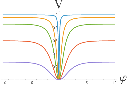
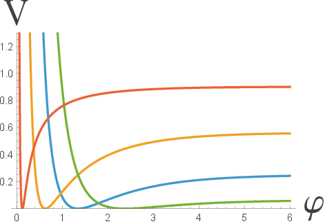
Think of the inflating universe like a ball rolling on a very flat, high plateau. The shape of that “landscape” (called the potential) decides what patterns inflation leaves in the sky.
- Exponential attractors: The plateau is approached extremely fast (like an edge that smooths out exponentially). These models famously predict and a very small that depends on another parameter, . Here, (about 50–60) is how long inflation lasts, measured in “e-folds.”
- Polynomial attractors: The plateau is approached more slowly, in a way that depends on a power (like ). These tend to give a slightly higher .
What the authors did:
- They started with the well-known “-attractor” setup (which naturally gives the exponential/plateau behavior).
- Then they replaced the simple plateau with a polynomial-shaped plateau controlled by μ and , but kept the same basic framework. This creates a single model that behaves like:
- An exponential attractor when μ is large.
- A polynomial attractor when μ is small.
They checked these behaviors with math (slow-roll approximations) and with numerical calculations, scanning different values of μ, , , and .
Main findings and why they matter
- Two-in-one behavior (a “double attractor”): For large μ, the model predicts the usual exponential -attractor results:
- (for , that’s about 0.964).
- (very small, and tunable by choosing ).
- For small μ, the same model predicts the polynomial attractor results:
- is a bit larger (for , around 0.972 or higher, depending on and μ).
- remains small and depends on μ and .
Together, by sliding μ, the models smoothly cover a wide band of values:
- For , about 0.9636 to 0.9818.
- This band comfortably includes the CMB-only results and the slightly higher suggested when combining CMB with DESI data.
The authors also show specific examples:
- With , , : for μ > 3, (exponential regime); for μ < 0.3, (polynomial regime).
In short, the new models act like a dimmer switch between two classic types of inflation behavior, letting researchers match current and future data more flexibly.
Implications and potential impact
- Unification: Instead of choosing either exponential or polynomial models, scientists can use one unified framework and adjust μ to fit observations.
- Data readiness: As measurements of and become more precise, these models can adapt without changing the overall theory.
- Testing inflation: The ability to tune across the observed range—while keeping predictably small—makes these models strong candidates for confronting upcoming CMB and galaxy survey data.
Key terms explained
- Inflation: A very early, ultra-fast expansion of the universe that smoothed things out and created tiny ripples we can still see.
- CMB (cosmic microwave background): The afterglow of the Big Bang, a baby picture of the universe that records those ripples.
- DESI: A project that maps galaxies to learn about the universe’s expansion and structure.
- Spectral index (): A number that tells us how the sizes of the ripples compare. If , slightly larger ripples are a bit weaker than smaller ones; typical models predict just below 1.
- Tensor-to-scalar ratio (): Tells how strong gravitational-wave ripples were compared to ordinary ripples; smaller means weaker gravitational waves from inflation.
- E-fold (): A way to measure the length of inflation; –$60$ means the expansion doubled about 50–60 times (on a logarithmic scale).
- Attractor: A model where many different starting points lead to the same predictions, making results robust.
- -attractor: A popular class of inflation models with a flat “plateau” shape that naturally gives stable predictions.
- μ (mu): The “slider” that moves the model between exponential-like and polynomial-like behavior.
- : A power that controls how fast the plateau is approached in the polynomial case.
In one sentence
This paper builds a simple, flexible family of inflation models that smoothly shifts between exponential and polynomial predictions by tuning one parameter, μ, letting the theory match a broad range of current and future cosmic data.
Knowledge Gaps
Knowledge gaps, limitations, and open questions
Below is a focused list of what remains missing, uncertain, or unexplored in the paper, phrased to be actionable for future work:
- Analytic interpolation: Derive closed-form (or controlled asymptotic) expressions for and in the intermediate- regime, beyond the two limiting cases and a single numerical example.
- Systematic parameter mapping: Provide comprehensive scans of showing the full footprint, including contours for different , to delineate which regions match current and forecast constraints.
- Reheating dependence of : Quantify how realistic reheating histories (equation-of-state, duration, temperature) shift and modify and across the interpolation; propagate reheating uncertainties into parameter constraints.
- Amplitude normalization: Compute across the parameter space to determine and the implied inflationary energy scale and Hubble rate; check consistency with bounds from particle physics and quantum gravity.
- Tensor sector: Characterize across the interpolation and identify regions compatible with current and near-future limits; verify whether the single-field consistency relation holds throughout.
- Running and higher-order slow-roll: Calculate the running (and possibly ) in both limits and across the transition to assess distinguishability from other models and consistency with data.
- Non-Gaussianity: Evaluate (and shapes) in the small-, intermediate, and large- regimes; assess whether transient features near the interpolation induce enhanced or feature-type non-Gaussianity.
- Transition dynamics: Analyze whether the -driven interpolation induces transient departures from slow roll (e.g., ultra–slow-roll episodes or inflection-like dynamics) and their imprints on the power spectrum and bispectrum.
- Initial conditions and overshoot: Assess the basin of attraction and overshoot risks, especially in the small- regime where the last 50–60 e-folds occur at ; quantify the fraction of initial conditions that lead to successful inflation.
- Stability near : Provide explicit regularizations for potentials with (where derivatives at the minimum can be singular) and verify that predictions for and remain robust under these regularizations.
- SUGRA embedding details: Construct explicit Kähler potential and superpotential realizations for both potential families, demonstrate stabilization of all orthogonal directions (including the imaginary component), and ensure mass hierarchies compatible with single-field dynamics.
- Quantum corrections and radiative stability: Compute loop corrections (and possible higher-derivative terms) on the hyperbolic field space to test the technical naturalness of the interpolation parameter and the stability of the plateau across regimes.
- Microphysical origin of : Identify the microscopic source of (e.g., moduli vevs, non-perturbative scales) in supergravity or string setups, determine its expected range/distribution, and assess fine-tuning (if any) required to match data.
- Swampland and distance conjectures: Evaluate field excursions and the role of negative curvature in the moduli space against swampland criteria; identify which regions are consistent with these bounds.
- Reheating dynamics and post-inflationary oscillations: Determine the inflaton mass at the minimum and the effective equation of state during reheating for each potential; connect these to reheating temperatures and .
- Vacuum structure and SUSY breaking: Specify the vacuum energy after inflation (Minkowski vs. dS) and outline how SUSY breaking is incorporated without destabilizing the inflationary trajectory or altering predictions.
- Potential pathologies and domain restrictions: For (with a barrier at ), analyze the domain of valid field values in the -attractor embedding (tanh map), and verify the absence of singularities or numerical instabilities in cosmological evolution.
- Degeneracies with late-time cosmology: Given the CMB–DESI tension under CDM, perform joint fits allowing both inflationary parameters and extended late-time parameters (e.g., , , curvature) to test whether the preference for small is robust.
- Bayesian data analysis: Replace qualitative coverage arguments with full likelihood analyses against Planck/ACT/SPT-3G + DESI (and BAO/SN) to locate the posterior over , including priors reflecting microphysical expectations.
- Forecasts and model discrimination: Produce forecasts (e.g., for CMB-S4, LiteBIRD, DESI final, Euclid) indicating how well future measurements of , , , and can distinguish polynomial vs. exponential regimes and pin down .
- Generality of “polyattractor” class: Provide a broader classification or necessary/sufficient conditions for double-attractor behavior beyond the two explicit potential families; identify whether other functional forms yield the same interpolation.
- Multi-field extensions: Explore whether mild couplings to additional light fields (curved trajectories, isocurvature, turns) spoil or preserve the double-attractor predictions and whether new observables emerge in the interpolation.
- Robustness to higher- and non-integer : Investigate predictions for a wider range of (including fractional values) and check whether numerical stability and observational viability persist.
- Eternal inflation and measure issues: Determine whether either regime (especially in the plateau limit) supports eternal inflation and whether that affects naturalness or measure-based predictions for .
- Numerical reproducibility: Document numerical methods, initial condition choices, and codes used for the checks (e.g., for ) to enable independent validation and extension to broader parameter regions.
Practical Applications
Overview
The paper introduces “polyattractors”: a simple, single-field α‑attractor family whose inflationary predictions continuously interpolate between exponential (plateau) and polynomial attractors by tuning an interpolation parameter μ. This yields a controlled mapping from model parameters (μ, α, k, N) to observables (ns, r), covering the range 1 − 2/N ≤ ns ≤ 1 − 1/N (e.g., 0.9636 < ns < 0.9818 for N = 55) and accommodating both CMB-only and CMB+DESI-preferred values. Below are actionable applications, organized by near-term and longer-term horizons.
Immediate Applications
- Incorporate polyattractor priors in cosmological parameter estimation
- Sector: academia; software; survey collaborations (e.g., Planck, ACT, SPT‑3G, DESI).
- What to do: Add μ (plus α, k) as model parameters in inference frameworks (Cobaya, MontePython) and use analytic mappings ns(N, μ, α, k) and r(N, μ, α, k) to set informative priors for inflation. Run MCMC/BNNs to obtain posteriors for μ and α from current CMB+BAO data.
- Tools/workflows: CAMB/CLASS + Cobaya/MontePython; JAX/NumPyro-based samplers; likelihood combo (Planck/ACT/SPT/DESI).
- Dependencies/assumptions: ΛCDM baseline in current likelihoods; slow-roll, single-field dynamics; N prior (reheating-dependent); DESI DR2–CMB tension could be due to systematics.
- Rapid tension diagnostics between CMB and DESI using μ as a “bridge” parameter
- Sector: academia; policy (survey working groups and advisory panels).
- What to do: Test whether allowing μ to vary resolves or reduces the CMB–DESI tension in ns under ΛCDM by comparing Bayes factors and information criteria (AIC/BIC) across μ regimes.
- Tools/workflows: Model selection modules; posterior predictive checks; tension metrics (e.g., Suspiciousness, Parameter Difference).
- Dependencies/assumptions: Tension may persist if driven by non-inflationary systematics; model comparison sensitive to priors on μ and N.
- Forecast discrimination power of upcoming missions for the “double-attractor” regimes
- Sector: academia; policy; instrument design (LiteBIRD, Simons Observatory, CMB‑S4).
- What to do: Use the derived ns and r scalings to quantify whether precise ns (δns ≲ 0.002) or B‑mode sensitivity (σ(r) ≲ 10−3–10−4) offers better leverage to distinguish small‑μ (polynomial regime) from large‑μ (exponential regime).
- Tools/workflows: Fisher forecasts; survey simulators; requirement calculators for r sensitivity and lensing delensing goals.
- Dependencies/assumptions: Achievable delensing; foreground complexity; true r may be very small in the polynomial regime.
- Update instrument requirement documents using model-driven targets
- Sector: policy; industry (detector manufacturers, cryogenics, readout electronics).
- What to do: Translate r = 12α/N2 (large μ) and r ∝ μ2k/(k+2) (small μ) into minimum sensitivity targets and sky coverage to guarantee regime discrimination. Prioritize spectral coverage and delensing capability accordingly.
- Tools/workflows: r–sensitivity calculators; cost–capability trade studies; schedule/integration planning.
- Dependencies/assumptions: Stable foreground removal; operational constraints; α and k choices affect r projections.
- Add polyattractor potentials to public theory+forecast libraries
- Sector: software; academia.
- What to do: Release a lightweight package providing V(φ) and V(ϕ) for the introduced Lagrangians, mapping {μ, α, k, N} → {ns, r}, with Jupyter examples and ready-to-plug modules for CLASS/CAMB.
- Tools/products: Python/Julia packages; JAX differentiable implementations for gradient-based sampling; Dockerized demos.
- Dependencies/assumptions: Community adoption; documentation and validation against existing results.
- Interactive “μ‑slider” educational and outreach tool
- Sector: education; public outreach.
- What to do: Build a web app where users vary μ, α, k and see in real time the potential shape, predicted ns and r, and where current data lie. Useful for teaching inflationary attractors and data-model interplay.
- Tools/products: WebGL/D3.js; Binder-hosted notebooks.
- Dependencies/assumptions: Accurate but simplified mappings; clear caveats about reheating/N.
- Model-building templates for SUGRA/string embeddings
- Sector: academia (theory).
- What to do: Use the paper’s supergravity-compatible forms to construct UV models with tuned μ that realize desired ns and r, leveraging disk/hyperbolic geometry (α control) and polynomial limits.
- Tools/workflows: Symbolic model builders; landscape scans; consistency checks (stability, reheating).
- Dependencies/assumptions: Valid effective field theory regime; control of higher-order corrections; isocurvature suppression.
- ML emulators for fast scans over μ, α, k, N
- Sector: software; academia; HPC/cloud industry.
- What to do: Train surrogates to map polyattractor parameters to observables and to likelihood/posterior summaries for ultra-fast forecasting and survey optimization loops.
- Tools/workflows: Gaussian processes/normalizing flows; ONNX deployment; HPC batch pipelines.
- Dependencies/assumptions: Training coverage; extrapolation risks; stable likelihood approximations.
- Curricular updates for advanced cosmology courses
- Sector: education.
- What to do: Integrate polyattractors as a unifying framework in lectures on inflationary phenomenology, showcasing how a single family spans benchmark predictions (Starobinsky-like to polynomial).
- Tools/products: Lecture notes; problem sets with reproducible code.
- Dependencies/assumptions: Pedagogical scaffolding on α‑attractors and slow-roll basics.
Long-Term Applications
- Regime selection via precision measurements of ns and r
- Sector: academia; policy; survey collaborations.
- What to do: Use next-generation constraints on ns (δns ~ 0.001–0.002) and r (σ(r) ~ 10−3 or better) to localize μ (small vs large), thereby testing the “double‑attractor” hypothesis and narrowing inflationary physics.
- Dependencies/assumptions: Mission delivery as planned; systematic control; reliable delensing.
- Reheating inference coupled to polyattractor fits
- Sector: academia.
- What to do: Jointly infer μ and reheating parameters (wreh, Treh) given their impact on N and thus on ns; build hierarchical models to separate inflationary vs reheating uncertainties.
- Dependencies/assumptions: Parametric reheating models; external priors (BBN, Neff); weak degeneracies with running.
- Strategic prioritization of B‑mode vs temperature/BAO improvements
- Sector: policy; funding agencies.
- What to do: If posteriors favor small μ, r may be suppressed, implying higher payoff from ns precision (temperature/BAO/LSS). If large μ is favored, B‑mode investment remains pivotal. Use decision analysis to guide funding allocations.
- Dependencies/assumptions: Stability of μ posteriors under new data; opportunity costs across facilities.
- Cross‑survey design optimization (CMB–LSS synergy)
- Sector: policy; academia; industry (technology integrators).
- What to do: Optimize joint strategies (sky overlap, redshift ranges, calibration standards) to tighten ns and break degeneracies (e.g., with Ωb, Neff), enhancing μ constraints.
- Dependencies/assumptions: Coordination across projects; interoperable data formats; calibration pipelines.
- UV completions and consistency tests in supergravity/string theory
- Sector: academia (theory).
- What to do: Embed polyattractors in controlled compactifications, exploring how α and μ arise from moduli geometry and stabilization, and what this implies for related observables (non‑Gaussianity, isocurvature).
- Dependencies/assumptions: Control of quantum corrections; explicit constructions with stabilizing mechanisms.
- Extended observable predictions beyond ns and r
- Sector: academia.
- What to do: Compute and constrain higher-order signatures (running αs, running of running) and reheating‑dependent imprints that could differ subtly between regimes, enabling sharper tests.
- Dependencies/assumptions: Sufficient observational precision; robust modeling of systematics.
- Standardization of inflation model repositories
- Sector: software; academia.
- What to do: Include polyattractors in community “inflation model zoos” with standardized APIs, metadata, reference implementations, and validation suites to improve reproducibility and interoperability.
- Dependencies/assumptions: Community governance; maintenance commitments.
- Informing next‑gen gravitational wave experiment priorities
- Sector: policy; industry.
- What to do: Use the r forecasts from polyattractor regimes to evaluate feasibility and science return of ultra‑low‑r searches and to set realistic targets for space and ground concepts beyond CMB‑S4/LiteBIRD.
- Dependencies/assumptions: Foreground floor; achievable delensing; cost constraints.
- Public engagement and literacy on data–theory iteration
- Sector: education; public outreach.
- What to do: Use the μ‑interpolation narrative to explain how theory adapts to data and how new surveys guide parameter spaces, improving public understanding of scientific method and investment rationale.
- Dependencies/assumptions: Effective science communication channels; accessible visuals.
Cross-cutting assumptions and dependencies
- Single-field, slow-roll α‑attractor dynamics with canonical inflaton in the canonically normalized variable and specific field-space geometry; negligible isocurvature and small non‑Gaussianity.
- Number of e‑folds N depends on reheating; priors on N materially affect ns predictions.
- Current tensions (e.g., DESI DR2 vs CMB) may involve unmodeled systematics under ΛCDM; resolving them could shift preferred μ.
- Degeneracies with extended cosmologies (Neff, Yp, running αs) need careful treatment to avoid misattributing effects to μ.
- Practical impact on instrument design hinges on realistic delensing and foreground mitigation.
Glossary
- ACT: The Atacama Cosmology Telescope, a ground-based experiment measuring the CMB to test cosmological models. "The tension with ACT is ,"
- α-attractors: A class of inflationary models with hyperbolic field-space geometry that yield universal predictions parameterized by α. "In the new -attractor models introduced in our paper,"
- BAO: Baryon Acoustic Oscillations, imprints of sound waves in the early universe used as a standard ruler in large-scale structure. "CMB and BAO data."
- CMB: The Cosmic Microwave Background, relic radiation from the early universe that constrains inflationary models. "CMB result "
- Canonically normalized inflaton field: A field redefinition giving a standard kinetic term, simplifying dynamics and predictions. "as the canonically normalized inflaton field increases."
- DESI DR2: The second data release of the Dark Energy Spectroscopic Instrument, providing precise clustering data. "the recent DESI DR2 data"
- Disk variables: Complex coordinates on the unit disk used to parametrize the α-attractor field space. "In disk variables , this model is"
- e-foldings: Logarithmic measure of expansion during inflation; N counts the number of exponential growth factors. "last O(60) e-foldings of inflation"
- Exponential α-attractors: Subclass of α-attractors where the potential approaches a plateau exponentially in the canonical field. "exponential -attractors"
- Higgs inflation: An inflationary scenario where the Standard Model Higgs field acts as the inflaton, often via nonminimal coupling. "the Higgs inflation"
- Inflationary attractors: Families of inflation models with universal observational predictions largely insensitive to microphysical details. "There are two main classes of inflationary attractors, exponential and polynomial"
- Inflaton: The scalar field responsible for driving cosmic inflation through its potential energy. "inflaton field increases."
- ΛCDM: The standard cosmological model with a cosmological constant (Λ) and cold dark matter (CDM). "under the assumption of CDM."
- Moduli space: The space of scalar field parameters (moduli) in high-energy theories; in α-attractors it has a boundary. "boundary of the moduli space "
- Plateau potentials: Potentials that asymptote to a nearly constant value at large field, yielding robust inflation predictions. "These models have plateau potentials,"
- Polyattractors: α-attractor models that interpolate between polynomial and exponential attractor regimes by tuning parameters. "one may call them polyattractors."
- Polynomial attractors: Inflationary models where the plateau is approached via power-law (polynomial) corrections in the field. "class of polynomial attractors"
- Slow-roll predictions: Approximate analytic predictions for observables assuming the inflaton rolls slowly down its potential. "in agreement with the slow-roll predictions"
- Spectral index : Parameter describing the tilt of the primordial scalar power spectrum from scale invariance. "the spectral index for CMB + DESI becomes higher: "
- SPT-3G: The third-generation South Pole Telescope CMB experiment providing high-precision measurements. "when combined with SPT-3G, the tension increases"
- Starobinsky model: An gravity inflation model equivalent to an α-attractor with α≈1. "the predictions of the Starobinsky model"
- Supergravity: A theory combining supersymmetry with general relativity, used to construct consistent inflationary potentials. "In supergravity with canonically normalized fields "
- T-model: A specific α-attractor potential with tanh-shaped dependence of the canonical field. "the standard -attractor T-model potential"
- Tensor-to-scalar ratio : The ratio of primordial gravitational wave amplitude to scalar perturbations, a key inflation observable. "tensor-to-scalar ratio "