Relaxed Lagrange Multiplier (RLM) Schemes for Phase Field Models Preserving the Relaxed Original Energy Dissipation Law

Abstract: Phase-field models are typically derived from variational principles for a free-energy functional and are widely used to simulate complex multiphase phenomena in science and engineering. A central goal in designing numerical schemes for these models is to preserve the underlying energy-dissipation law. In this paper, we propose a class of relaxed Lagrange multiplier (RLM) schemes for phase field models. In contrast to popular scalar auxiliary variable (SAV) and invariant energy quadratization (IEQ) methods, which dissipate a modified energy involving auxiliary variables, the RLM schemes dissipate a relaxed version of the original energy and closely track the original energy dissipation rate. Compared with the classical Lagrange multiplier (LM) approach, the RLM schemes ensure that the resulting discrete system is uniquely solvable over a broad range of time steps. The key idea is to augment the LM formulation with a relaxation term, yielding a scalar quadratic equation for the multiplier with an explicit closed-form solution. The resulting schemes are linear and efficient because each time step requires solving only two linear systems with constant coefficients, at a cost comparable to that of SAV schemes. We construct both first-order and second-order variants and prove their energy stability. Numerical experiments verify the expected convergence rates and demonstrate that the RLM schemes accurately capture interface dynamics.

• The paper presents the RLM framework that embeds a relaxation parameter into the Lagrange multiplier approach to preserve the original energy dissipation law.
• It employs linear implicit time integration and quadratic scalar updates to achieve unconditional energy stability and computational efficiency.
• Numerical experiments show that the method is robust for singular energies and versatile across both Allen–Cahn and Cahn–Hilliard dynamics.

Relaxed Lagrange Multiplier Schemes Preserving the Relaxed Original Energy Dissipation Law

Introduction and Context

The paper "Relaxed Lagrange Multiplier (RLM) Schemes for Phase Field Models Preserving the Relaxed Original Energy Dissipation Law" (2607.00355) addresses the design of structure-preserving, efficient, and linear time integration methods for phase field models, with an emphasis on accurately tracking the original free energy dissipation law while ensuring unique solvability and computational tractability. Traditional approaches such as scalar auxiliary variable (SAV) and invariant energy quadratization (IEQ) schemes only track modified energies, whereas direct Lagrange multiplier (LM) formulations guarantee original energy dissipation but confront nonlinear, possibly ill-posed, algebraic equations for the multiplier. The RLM framework seeks to bridge this gap by embedding a relaxation mechanism into the LM method, yielding an energy dissipation law that approximates the original free energy with high accuracy, without the challenging nonlinear solver bottleneck.

Formulation: The RLM Framework

The RLM method introduces a scalar relaxation parameter $\alpha$ into the temporal discrete energy law. The phase field PDE and associated discrete-time schemes are rewritten to include a multiplier $q^{n+1}$ and a penalty term $\alpha[q^{n+1,2}-(q^n)^2]$, yielding a "relaxed original" energy

$\widetilde{E} = E + \alpha (q^2 - 1),$

where $E$ is the original free energy. For moderate or large $\alpha$ and well-chosen $q^{n+1}$, the scheme guarantees

$\widetilde{E}^{n+1} - \widetilde{E}^n \leq 0,$

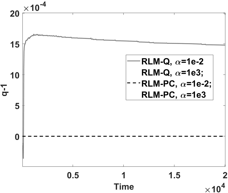
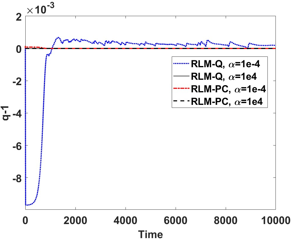
thus enforcing unconditional energy stability at the discrete level. In contrast to SAV/IEQ, the dissipation law is expressed in the physical variables, and for sufficiently large $\alpha$, the relaxation penalty enforces $q \approx 1$, driving $q^{n+1}$0.

Crucially, the relaxation converts the nonlinear scalar equation for $q^{n+1}$1 encountered in LM schemes into a quadratic one (or, for some variants, a simple closed-form update), which can be solved explicitly and robustly at each time step.

Numerical Schemes: RLM Variants

The core algorithms are first- and second-order accurate temporal schemes, presented as RLM-BDF1 (Backward Differentiation Formula) and RLM-CN (Crank–Nicolson), each of which consists, per time step, of:

1. Two linear solves for the state variables (with constant-coefficient operators),
2. Solution of a quadratic scalar equation for $q^{n+1}$2.

Two main practical variants are analyzed in detail:

• RLM-Q (Quadratization): The nonlinear free energy is approximated by a quadratic surrogate, ensuring the multiplier equation is explicitly quadratic with known discriminant structure. For sufficiently large $q^{n+1}$3, there is a unique positive solution for $q^{n+1}$4. See (Figure 1).

Figure 2: Solution structure of the RLM-Q quadratic scalar equation for the multiplier $q^{n+1}$5, identifying the unique stable branch as a function of $q^{n+1}$6.

• RLM-PC (Prediction-Correction): The multiplier update is based on a predicted state (with $q^{n+1}$7), leading to an even simpler quadratic for $q^{n+1}$8. Robustness is enhanced, especially when the quadratic surrogate is inaccurate or for stiff potentials.

For both variants, the schemes remain linear, allowing efficient FFT-based or sparse direct solvers in combination with constant-coefficient Laplacians or elliptic operators.

Analysis: Properties, Stability, and Solvability

Energy Stability: Both first- and second-order schemes are rigorously proved to be unconditionally energy stable with respect to the relaxed original energy $q^{n+1}$9, under general phase field functionals and both Allen–Cahn (non-conserved) and Cahn–Hilliard (conserved) dynamics.

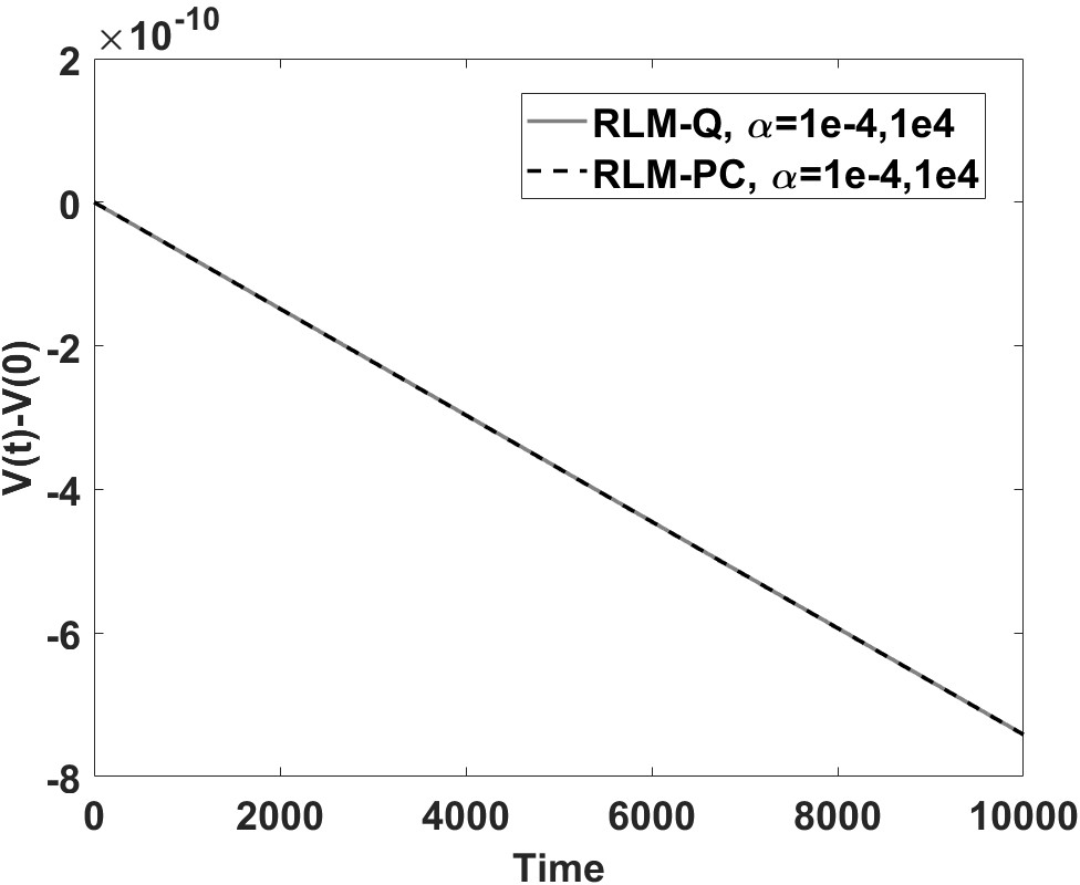
Mass Conservation: For mass-conserving flows (e.g., Cahn–Hilliard), the RLM system preserves total integral mass exactly under appropriate boundary conditions, as the relaxation only enters the chemical potential, not the mass-conserving spatial operator.

Solvability: For finite $\alpha[q^{n+1,2}-(q^n)^2]$0, the quadratic equation for $\alpha[q^{n+1,2}-(q^n)^2]$1 is always solvable for sufficiently large $\alpha[q^{n+1,2}-(q^n)^2]$2; the discriminant and uniqueness are characterized by closed-form expressions. The positive root closest to $\alpha[q^{n+1,2}-(q^n)^2]$3 is selected, ensuring continuity and adherence to the physical dynamics.

Consistency and Error: As $\alpha[q^{n+1,2}-(q^n)^2]$4 and $\alpha[q^{n+1,2}-(q^n)^2]$5, $\alpha[q^{n+1,2}-(q^n)^2]$6 and $\alpha[q^{n+1,2}-(q^n)^2]$7; thus, the RLM framework recovers the physical dissipation law. Practically, even moderate $\alpha[q^{n+1,2}-(q^n)^2]$8 suffices for fidelity. Modeling and truncation errors introduced by the regularization are controlled and shown to be $\alpha[q^{n+1,2}-(q^n)^2]$9, where $\widetilde{E} = E + \alpha (q^2 - 1),$0 is the temporal order.

Numerical Experiments: Accuracy and Efficiency

A comprehensive suite of experiments is given across Allen–Cahn, Cahn–Hilliard, and conserved Allen–Cahn models, with polynomial, logarithmic (Flory-Huggins), and singular (Lennard–Jones-type) free energy densities.

• Temporal Accuracy: Both RLM-Q and RLM-PC achieve the expected first/second-order convergence rates; see error tables in the text.
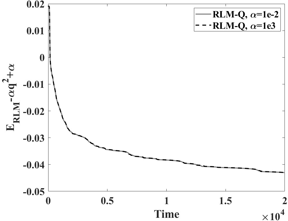
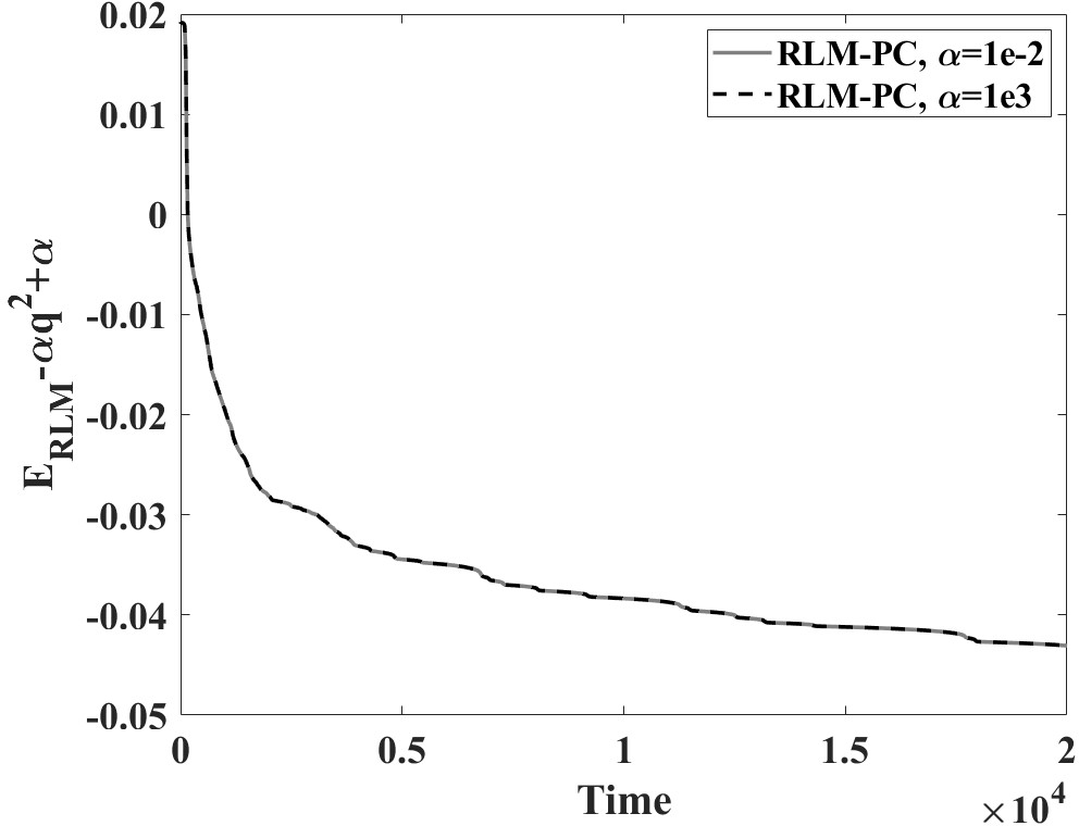
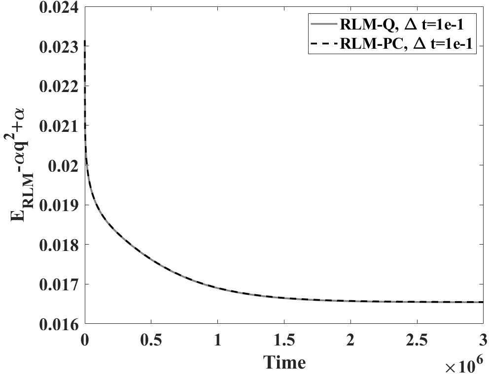
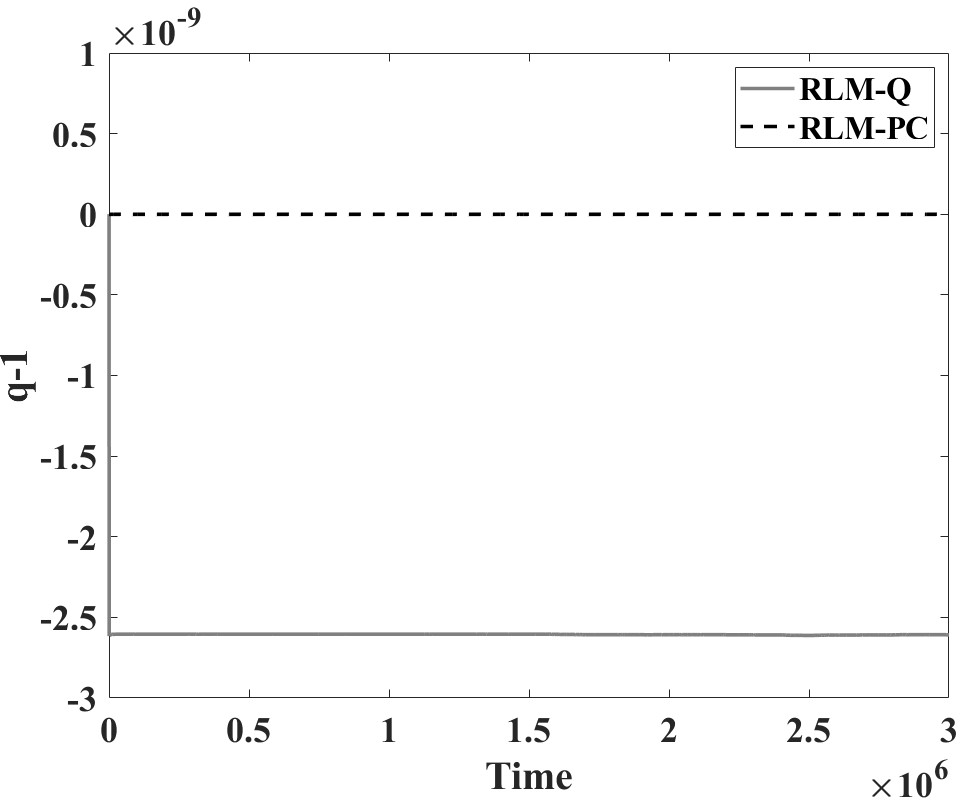
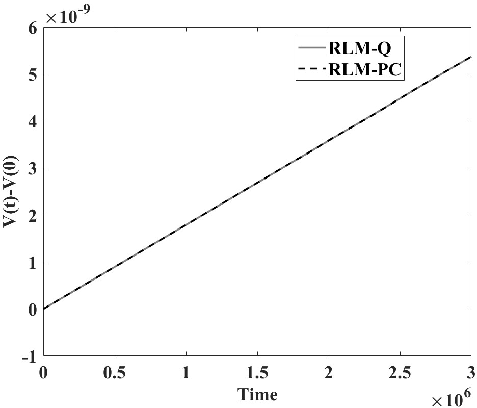
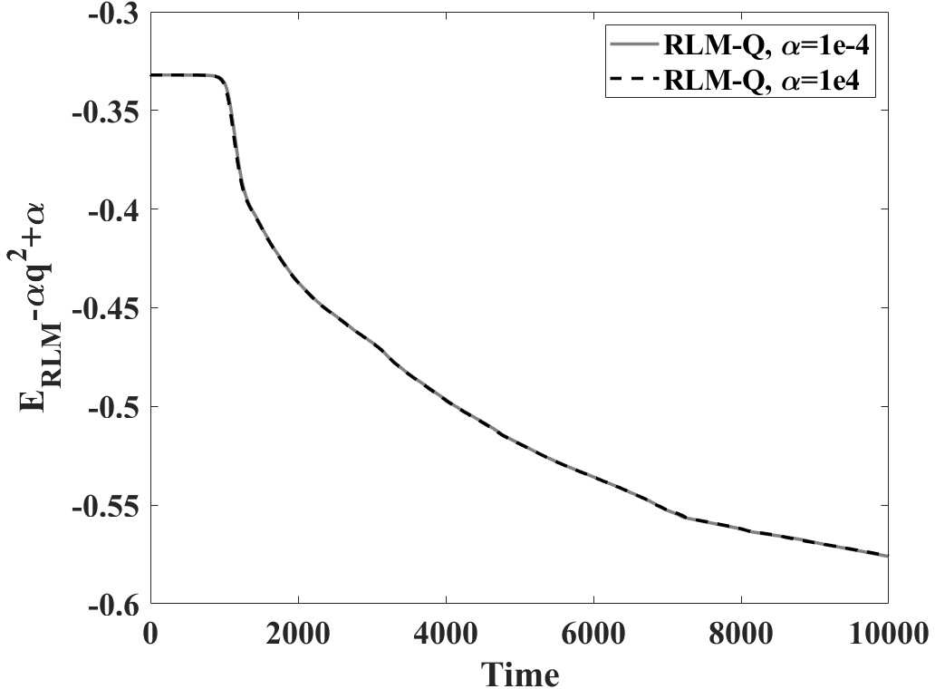
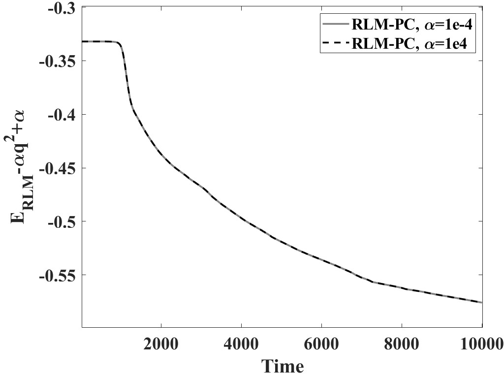
• Energy Dissipation: RLM closely tracks the original energy curve, with negligible discrepancy for moderate $\widetilde{E} = E + \alpha (q^2 - 1),$1. The deviation term $\widetilde{E} = E + \alpha (q^2 - 1),$2 is empirically $\widetilde{E} = E + \alpha (q^2 - 1),$3.
• Dynamics: Interface coarsening, droplet merging, and pattern formation scenarios were simulated. RLM schemes yield indistinguishable interface dynamics compared to SAV and IEQ for regular problems, but offer superior robustness and accuracy for singular energies where auxiliary-variable-based methods fail.

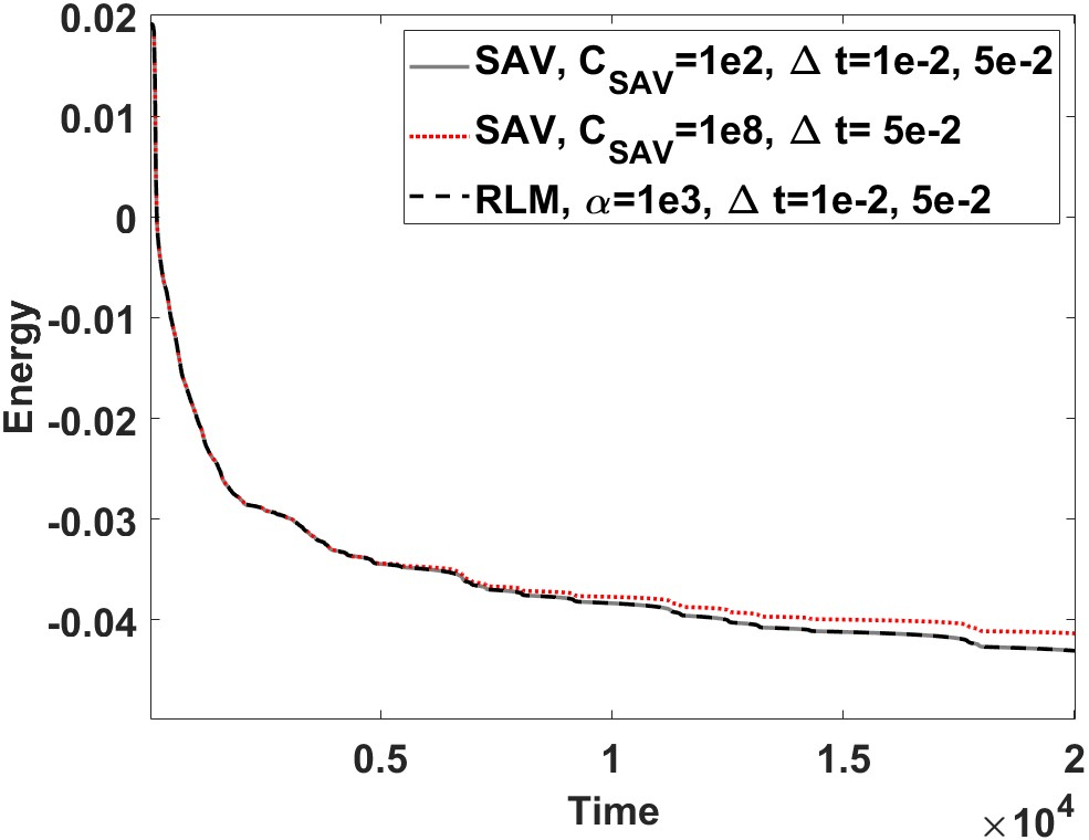
Figure 4: Evolution of the original energy, showcasing how RLM schemes match the energy decay rate of SAV/IEQ schemes while tracking the true energy more faithfully under relaxed dissipation.

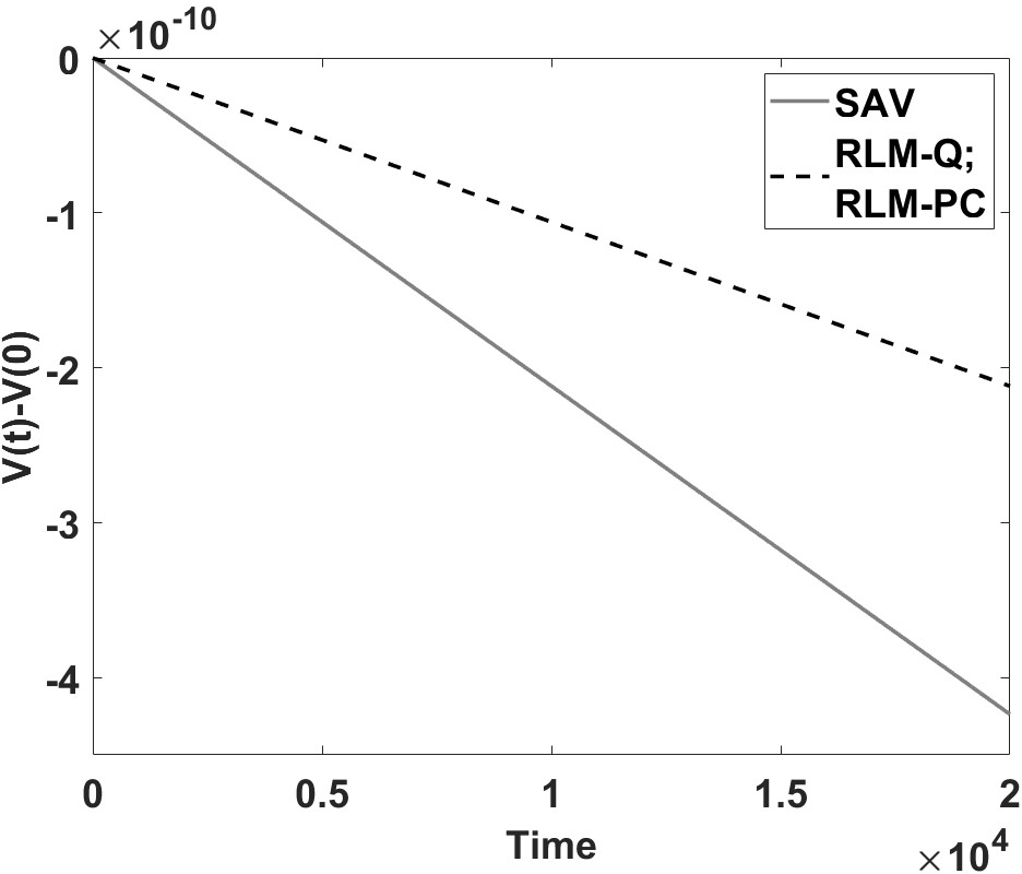
Figure 6: Detailed energy dissipation rates with varying $\widetilde{E} = E + \alpha (q^2 - 1),$4. The energy difference $\widetilde{E} = E + \alpha (q^2 - 1),$5 is minimized as $\widetilde{E} = E + \alpha (q^2 - 1),$6 increases, confirming control over numerical fidelity.

• Lennard–Jones-type Thin Films: Demonstrated well-posedness and energy decay tracking by RLM on a system where SAV’s square-root auxiliary variable cannot be defined due to singularities at $\widetilde{E} = E + \alpha (q^2 - 1),$7.

Figure 8: RLM-Q simulation results for a singular Lennard–Jones-type potential, demonstrating robust energy decay and $\widetilde{E} = E + \alpha (q^2 - 1),$8 under modest relaxation.

• Scaling and Robustness: SAV/IEQ require regularization constants tuned to each potential, and can be sensitive or inaccurate for stiff or unbounded energies. RLM, by contrast, is insensitive to such choices; its only tunable parameter $\widetilde{E} = E + \alpha (q^2 - 1),$9 can be problem-independent and large, ensuring universality and simplicity in deployment.

Implications and Future Directions

The RLM method delivers practical, robust, and linearly implicit time integration for a broad class of phase field models including those with singular energy densities. It guarantees unconditional energy stability and, with proper choice of $E$0, ensures the energy tracked is arbitrarily close to the original free energy. Unlike LM/SVM and other physical-variable schemes, which can become ill-posed or require nonlinear solves, RLM is always explicitly solvable, offering significant improvements in implementation and reliability.

Implications:

• Model Generality: RLM is applicable to higher-order, nonlocal, multi-component, and singular free energy systems without additional adaptation.
• Computational Efficiency: Single (or two) linear solves per timestep avoid Newton or fixed-point iterations, matching the efficiency of SAV/IEQ.
• Numerical Fidelity: The original energy functional is tracked up to relaxation error, unlike auxiliary variable schemes where dissipation is enforced only on a surrogate.

Future Directions:

• Extension to third- or higher-order temporal schemes and practical adaptive timestepping strategies.
• Application to coupled multiphysics (multi-order parameter, fluid-structure, etc) PDEs where structure preservation is essential.
• Development of a priori error bounds for $E$1 as a function of $E$2, mesh, and time step.
• Optimal selection of $E$3 balancing stability and numerical properties via adaptive procedure.

Conclusion

The RLM scheme advances the state of the art in structure-preserving, energy-stable numerical methods for phase field PDEs. By introducing a tunable relaxation mechanism, it circumvents the main drawbacks of the standard Lagrange multiplier/integral-constraint approaches, while achieving greater physical fidelity relative to auxiliary variable methods. The framework is rigorously analyzed, robust for singular potentials, easily implementable, efficient, and widely applicable to both standard and challenging free energy landscapes.