Trends, Volatility, Correlations, and Critical Phenomena in Financial Markets
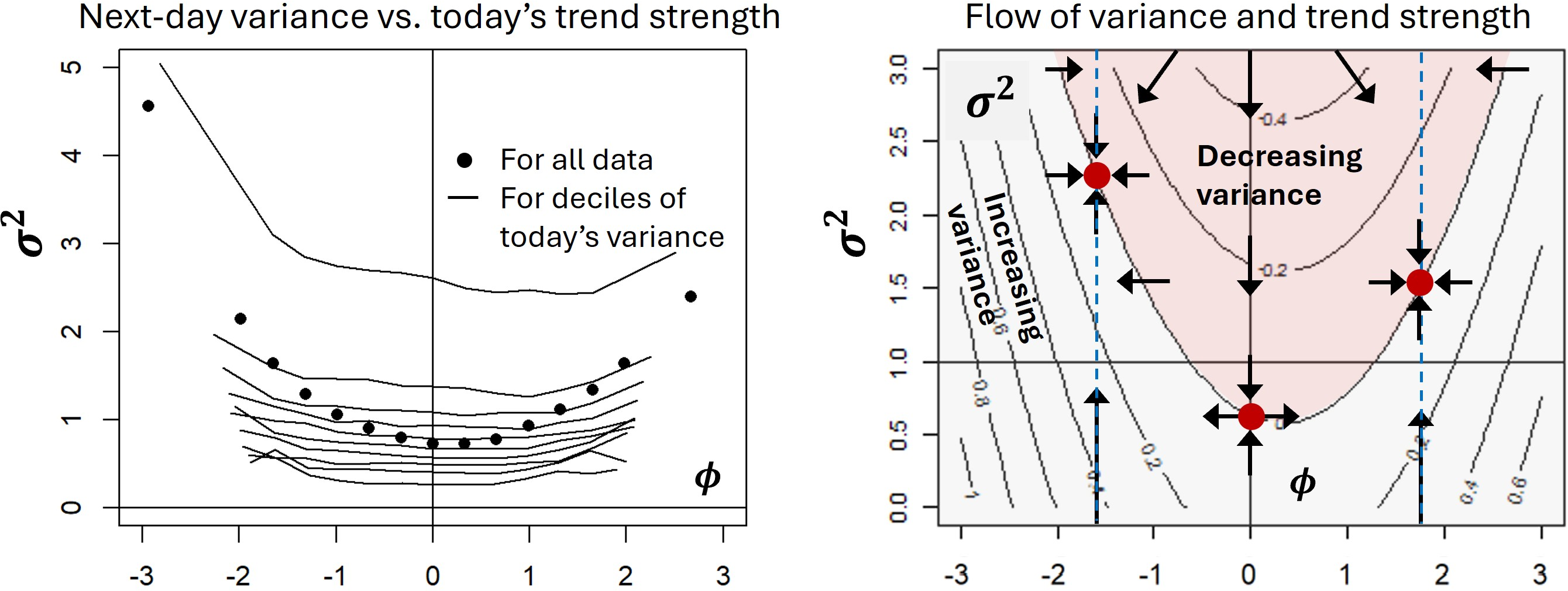
Abstract: We forecast future volatilities and correlations of financial markets based on the current trends in these markets. This complements previous work that models future expected returns by a cubic polynomial of the current trend strength. Empirically, we observe that volatilities and correlations tend to increase day after day in times of strong up- or down-trends. This effect is particularly pronounced in down-trends. It can be accurately quantified by quadratic polynomials of today's trend strengths, which refine common mean-reversion models of volatilities and correlations. Our results improve the prediction of market risk by accounting for market trends. They also support a recent proposal to model financial markets by a lattice gas near its critical point.
Paper Prompts
Sign up for free to create and run prompts on this paper.
Top Community Prompts
Explain it Like I'm 14
Overview: What this paper is about
This paper asks a simple question with big consequences for investing: can we predict how risky markets will be tomorrow by looking at how “trendy” they are today? The authors show that when prices are in strong up- or down-trends, market risk (how much prices swing) and how much markets move together (correlations) both tend to rise—especially during down-trends. They build simple, math-light rules to capture this and explain why it matters for managing risk and understanding how markets behave.
The key questions in plain language
The authors focus on five easy-to-grasp questions:
- Do strong trends today make tomorrow more volatile (bumpy)?
- Do strong trends make different markets move together more?
- Is this effect stronger in down-trending markets than in up-trends?
- Does the time scale of the trend (days vs months) matter?
- Can these facts help improve the models that investors use to measure and control risk?
How they studied it (methods explained simply)
The team analyzed 33 years of daily price data for 24 futures markets (covering stocks, bonds, currencies, and commodities) across 10 time horizons (from a couple of days to multiple years). They did three main things:
- Measuring trend strength Think of trend strength as “how strong and reliable the recent direction looks.” They turn this into a single number using a statistic that says how big the trend is compared to normal day-to-day wiggles (noise). Bigger number = clearer trend.
- Tracking risk with an everyday idea: recent averages matter most They measured “how bumpy” prices are (volatility) using an exponentially-weighted moving average (EWMA). That’s just a fancy way of saying: take an average, but give recent days more weight than older days.
- Seeing what predicts tomorrow They used simple equations (called regressions) to test what best predicts tomorrow’s:
- Volatility: today’s volatility plus how strong today’s trend is.
- Correlation between two markets: today’s correlation plus how strong each market’s trend is.
They also:
- Grouped (binned) days by similar trend strengths to visualize patterns.
- Used bootstrapping and cross-validation (ways to check their results aren’t just luck) to make sure the findings hold up on new data.
- Measured correlations mostly with weekly returns (to reduce timing issues from different closing hours in New York, Europe, and Asia).
What they found and why it matters
1) Trends raise volatility, especially in down-trends
- When markets are in strong up- or down-trends, tomorrow’s volatility tends to be higher.
- This is strongest when the trend is down. In other words, markets get more jittery when they’re falling fast. This is the “leverage effect” often seen in stocks.
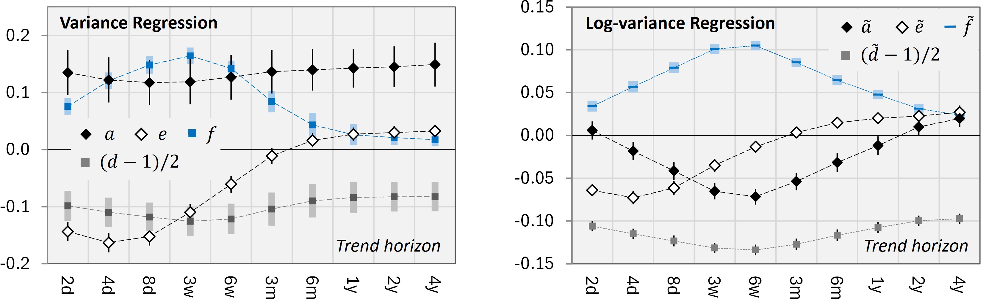
- Shorter-term trends (up to about 3 months) matter most for predicting tomorrow’s volatility.
Why this matters: Risk managers and traders should expect risk to climb during strong trends, especially during selloffs. That means bigger safety buffers may be needed.
2) Trends raise correlations: markets “move together” more in crises
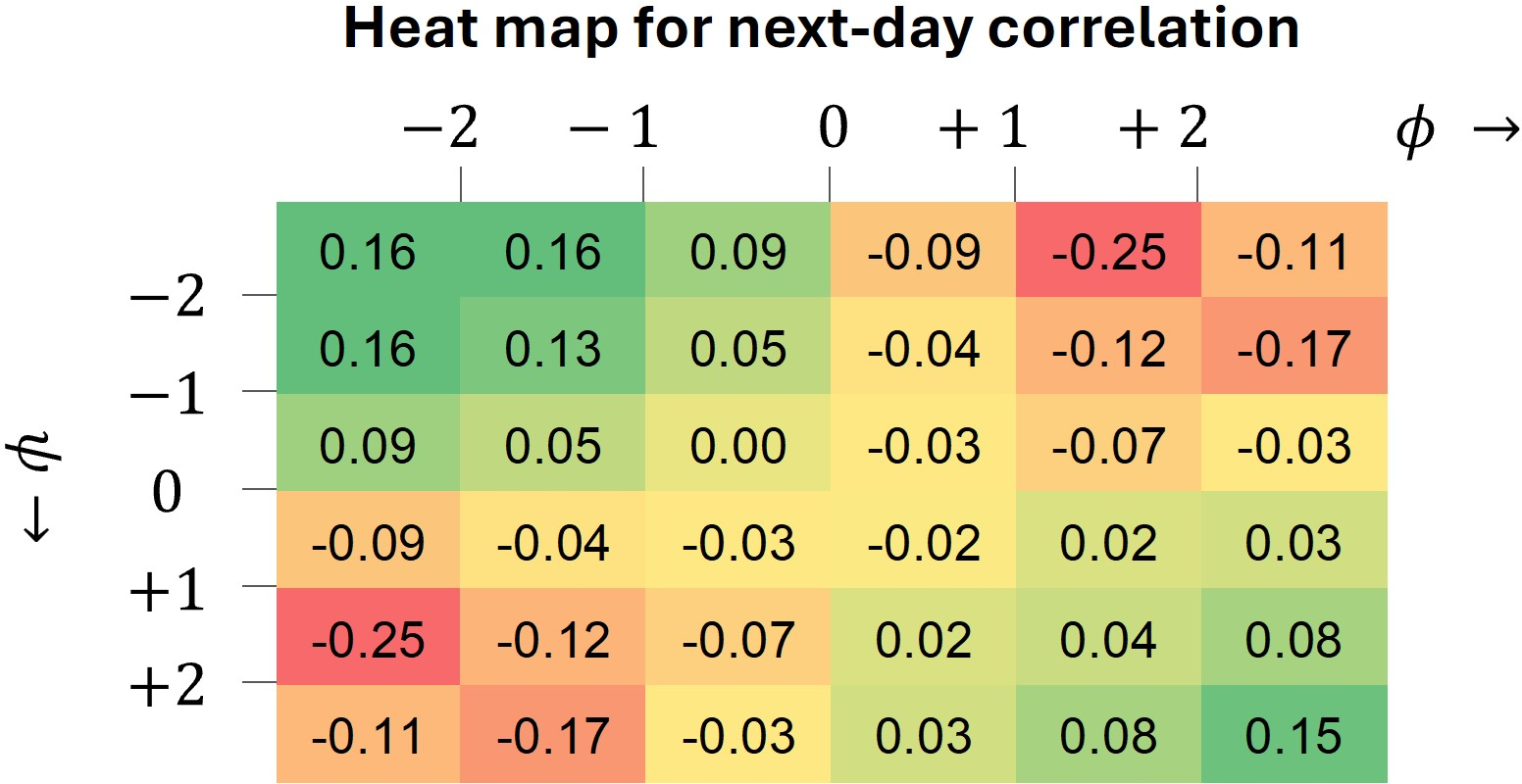
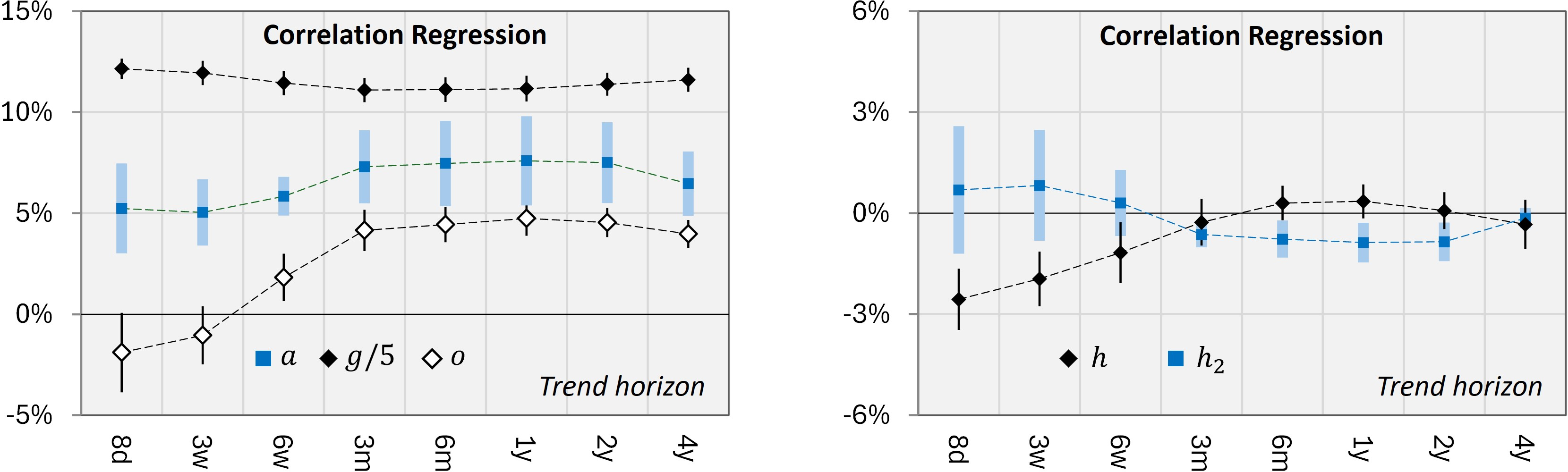
- When two markets both have strong trends in the same direction—especially both trending down—their returns next week are more correlated than usual.
- If one is trending up and the other down, their correlation tends to be lower than usual.
- Correlations “snap back” to normal fairly fast (they mean-revert), faster than volatility does.
Why this matters: In tough times, diversification can weaken because many risky assets fall together. Planning for this ahead of time can prevent nasty surprises when you most need protection.
3) Today still matters a lot for tomorrow
- Tomorrow’s volatility is strongly connected to today’s volatility (volatility clusters).
- Tomorrow’s correlation is strongly connected to today’s correlation.
- But adding “trend strength” improves the predictions in both cases.
Why this matters: Popular risk models that only look at past volatility/correlation miss an important signal—current trend. Adding it improves risk forecasts.
4) A different lens (log-volatility) tells the same story
- The authors also looked at “log-variance” (think: a curved ruler for measuring volatility) and found similar results: trend terms help explain changes in risk.
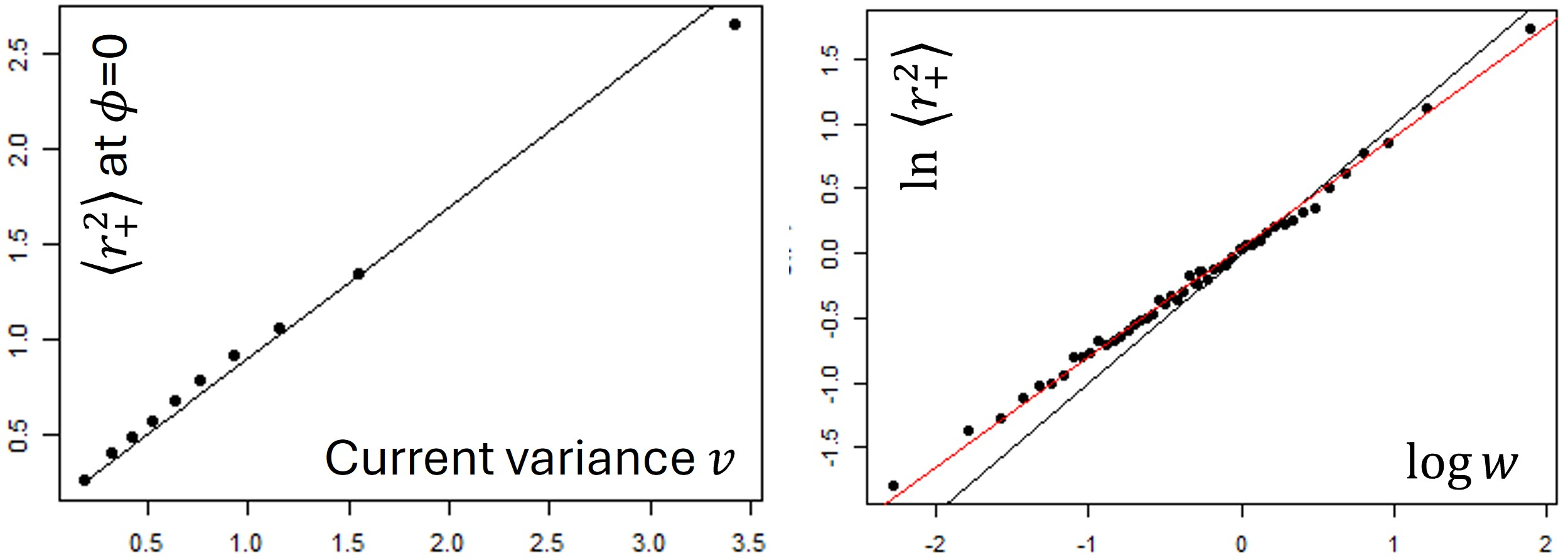
- Without trends, tomorrow’s variance grows roughly like today’s variance to the power of about 0.8–0.9, not quite linearly.
Why this matters: It shows the effects are robust, no matter which reasonable way you measure risk.
5) “Fat tails” are real, but not driven by trend strength alone
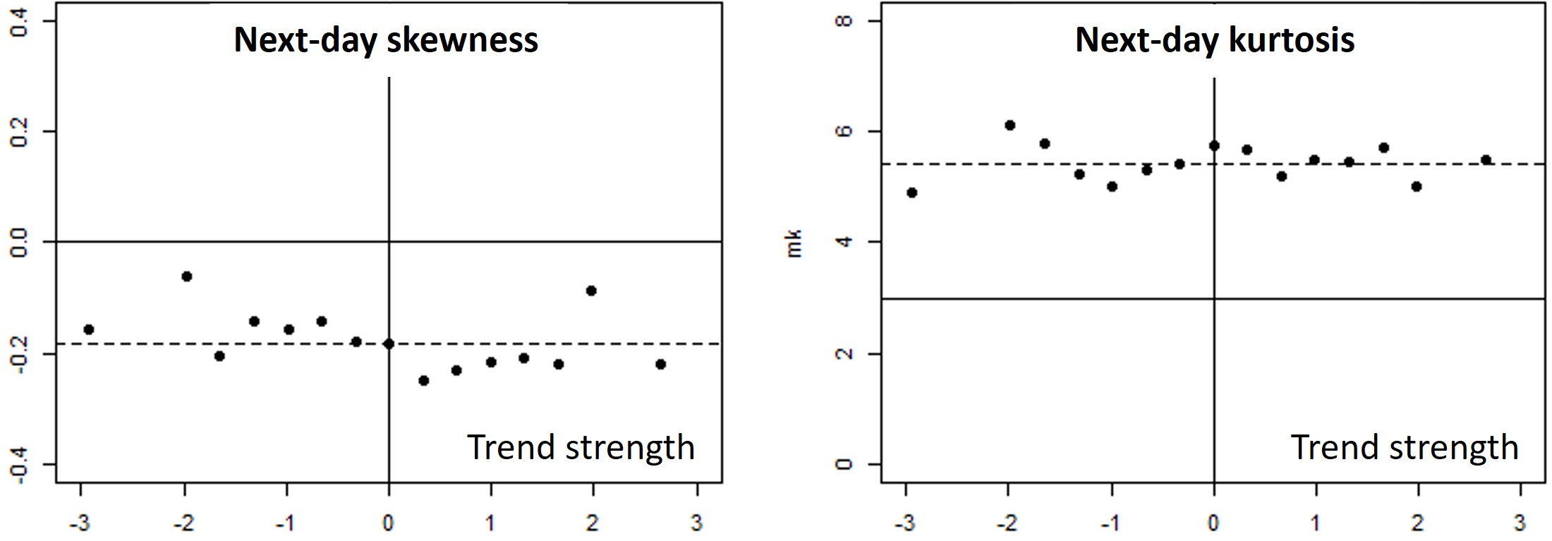
- Returns are lopsided and have “fat tails” (extreme moves happen more often than a normal bell curve would predict).
- However, within any single trend bucket, the “extra-peakiness” (kurtosis) doesn’t change much with trend.
- Mixing together days with different volatilities naturally creates fat tails overall—so just the fact that volatility changes over time explains a lot of the wildness we see.
Why this matters: Big, sudden moves are to be expected. Risk systems should assume that volatility shifts around and that this mixing creates heavy tails.
A simple picture of their models
- Volatility model: Tomorrow’s volatility = “pull back toward normal” + “what volatility is today” + “extra from trend strength,” where down-trends add more than up-trends.
- Correlation model: Next week’s correlation = “pull back toward normal” + “what correlation is today” + “extra when both markets trend the same way.”
Short horizons mainly drive volatility effects; longer horizons matter more for the “move together” effect.
Why this could be a big deal
- Better risk management: Portfolios can be made safer by adjusting risk limits when strong trends appear, especially during selloffs.
- More realistic models: Popular tools like GARCH or Heston (volatility models) can be improved by adding trend signals and asymmetry between up- and down-trends.
- Smarter diversification: Expect correlations to jump in crises; plan hedges and safe-haven assets accordingly.
A neat physics connection (optional intuition)
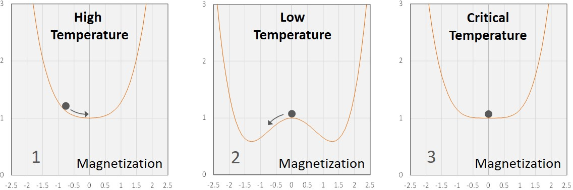
The authors relate markets to a physics model near a “critical point” (like water boiling). Near that point, small changes can cause big effects, and systems show patterns like those seen in markets (clustering, stronger co-movements, fat tails). In their analogy:
- Trend persistence and reversal behave like forces in a “potential” that pushes prices back when trends get too strong.
- A changing, complex network of investors acts like a dynamic surface that naturally produces changing volatility.
- This framework helps explain why down-trends pump up volatility (the leverage effect) and why correlations surge in crises.
You don’t need the physics to use the results—but it gives a deeper reason why these patterns appear.
Bottom line: what to remember
- Strong trends today often mean higher volatility tomorrow, especially in down-trends.
- When two markets trend together—particularly downward—they become more correlated.
- These effects are strongest at shorter trend horizons for volatility, and at longer horizons for “move together” behavior.
- Adding trend information to standard risk models makes them more reliable—especially when markets are stressed, which is exactly when better risk estimates matter most.
Knowledge Gaps
Unresolved gaps, limitations, and open questions
Below is a concise list of concrete gaps and open questions that remain after this study and that future research could address:
- Data scope and representativeness
- Generalizability beyond 24 liquid futures (e.g., single-stock equities, corporate bonds, EM assets, crypto, options) remains untested.
- Impact of contract roll, changing futures specifications, and benchmark transitions (e.g., euro introduction) on trend and volatility estimates is not controlled or stress-tested.
- Effects at intraday or higher-frequency horizons are not analyzed for variance/correlation despite earlier intraday return findings; results may differ materially.
- Non-synchronous trading and correlation measurement
- Weekly aggregation is used to mitigate non-synchronous closes, but this sacrifices information and may introduce biases; no comparison to synchronization methods (e.g., Hayashi–Yoshida, lead–lag adjustments, overlapping trading hours).
- The Epps effect and time-zone effects are not explicitly modeled; how much the reported trend–correlation effect survives under properly synchronized data is unknown.
- Trend-strength definition and sensitivity
- Trend strength is defined via t-statistics across 10 fixed horizons; robustness to alternative trend filters (moving averages, momentum signals, detrended price oscillators), volatility normalizations, or horizon grids is not assessed.
- Sensitivity to the EWMA decay (α = 1 − e−1/16) used for variance and correlation estimators is not reported; optimal α may differ by asset class and horizon.
- Model specification and functional-form risk
- Variance and correlation models rely on low-order polynomials in trend strength; nonparametric or semi-parametric alternatives (splines, GAMs), regime-switching, or ML methods could capture nonlinearities missed by polynomials.
- Correlation regression does not enforce bounds or positive semidefiniteness in a multi-asset setting; an open problem is to embed trend terms within bounded, PSD-preserving frameworks (e.g., Fisher/Z-transform, DCC-type, matrix-factor models).
- The approximation σ_{t+1} ≈ σ_t in the correlation’s standardized returns may bias coefficients; the magnitude of this approximation error across regimes is not fully quantified.
- Statistical inference and validation
- Reported out-of-sample R² values are small (variance ≈ 0.12 daily; correlations ≈ 0.03 weekly); economic significance for risk management is not demonstrated with VaR/ES backtests or forecast evaluation tests (e.g., Diebold–Mariano).
- Cross-validation uses 15-fold splits and bootstrap t-stats that may not respect time dependence; time-series–appropriate validation (rolling/blocked CV, expanding-window, pre/post-regime) and heteroskedasticity/autocorrelation-robust inference are not presented.
- Overlapping-return biases for multi-day variance forecasts and their impact on t-stats are not discussed.
- Stability, regimes, and heterogeneity
- Parameter stability across subperiods (e.g., dot-com, GFC, COVID-19) and structural breaks is not examined; whether coefficients drift with market structure/liquidity changes is unknown.
- Universality claims (e.g., return-cubic coefficients) are not re-validated for variance/correlation; a formal hierarchical/random-effects analysis of cross-asset heterogeneity is missing.
- The equity-specific strength of leverage and correlation asymmetries is documented but not decomposed further (regions/sectors, small vs large cap proxies, volatility regimes).
- Causality and mechanism
- The direction of causality between trends and future variance/correlation is not identified; both could be driven by latent factors (e.g., macro news, liquidity shocks). Instrumental-variable or event-study designs could help.
- The role of contemporaneous returns vs accumulated trends in driving leverage/asymmetry is not disentangled.
- Higher moments and tail risk
- Skewness and kurtosis show no strong dependence on trend strength, but statistical power and confidence intervals are not reported; conditional tail risk (e.g., ES at high confidence) conditional on trend remains unquantified.
- The mixture argument tying heavy tails to the distribution of trend strengths is illustrative; a formal mixture-of-variance model fitted and validated against tails (Hill plots, stability of tail index) is not provided.
- Joint covariance modeling for portfolios
- A coherent multivariate covariance forecast that jointly models variances and correlations with trend inputs (and guarantees PSD) is not developed; integration with existing DCC/GO-GARCH/HAR frameworks is left open.
- Alignment of forecast horizons (daily variance vs weekly correlations) for portfolio applications is unresolved; implications for multi-asset risk forecasting at daily/weekly/monthly horizons are not quantified.
- Log-variance formulation and estimation
- The log-variance model uses approximations (e.g., ln E[r²] vs E[ln r²]) subject to Jensen effects; a principled estimation approach (e.g., QMLE/state-space with Kalman/particle filters) could clarify parameter meaning and reduce bias.
- The observed power-law relationship E[r²|σ²] ≈ (σ²)κ with κ ≈ 0.8–0.9 lacks a theoretical explanation; is κ stable across assets/regimes?
- Extensions to cross-asset effects
- Variance models omit cross-asset spillovers and lead–lag effects; do strong trends in one asset/asset class predict variance in others (volatility contagion)?
- Correlation models include only same-time trend terms; lagged cross-trend terms, volatility levels, or macro states might improve fit and interpretability.
- Practical utility and implementation
- Claims of improved risk prediction are not backed by operational backtests (VaR exceptions, ES backtesting, coverage tests) or comparisons to baseline GARCH/DCC/GJR and realized-volatility models.
- No guidance on parameter recalibration frequency, real-time implementability, or transaction-cost/latency considerations for practitioners.
- Theoretical (lattice-gas/criticality) link
- The statistical-mechanical model reproduces the functional form only to first order; signs and magnitudes of coefficients (e.g., leverage/asymmetry parameters) are not derived and matched to data.
- Multi-asset generalization (to produce co-movements, cross-terms, and a valid covariance matrix) is not yet developed; mapping theoretical parameters (α, β, γ, Q) to empirically estimated coefficients is an open task.
- Conditions under which the criticality-based mechanisms dominate vs standard market microstructure or macro drivers are not specified or tested.
- Robustness and alternative benchmarks
- No head-to-head comparison with asymmetric GARCH variants (GJR-EGARCH), DCC/ADCC, realized-kernel volatility, or HAR-type models augmented with trend terms.
- Sensitivity to outliers and crisis periods (robust regression, downweighting) is not shown; heavy tails may distort OLS-type fits.
Addressing these points would help establish the robustness, economic significance, and theoretical underpinnings of trend-informed volatility and correlation forecasting, and enable deployment in coherent multi-asset risk models.
Practical Applications
Overview
Below are actionable, real-world applications that flow directly from the paper’s findings on trend-conditioned forecasts of returns, volatility, and correlations, including refinements to mean-reverting variance/correlation models and evidence supporting crisis-time co-movement. Each application includes sector linkage, potential tools/products/workflows, and feasibility caveats.
Immediate Applications
These can be deployed with modest engineering and model-governance effort using the paper’s regression specifications, existing data (daily prices; EWMA volatility/correlation), and standard risk infrastructure.
- Finance (buy-side): Portfolio risk and allocation
- Use trend-aware volatility forecasts for risk budgeting, volatility targeting, and leverage control.
- Tool/workflow: Add a volatility module that forecasts next-day (or multi-day) variance via
σ̂²_{t+1} = a + d·σ²_t + e·φ_t + f·φ_t², and optionally the log-variance version. Weight short horizons (days–3 months) more heavily for variance. - Sectors: Asset management, hedge funds (incl. CTAs), pensions, insurers, family offices.
- Assumptions/dependencies: φ is the t-stat of trend over horizon T; coefficients are modestly time-varying and should be re-calibrated; leverage effect asymmetric (strongest in equities); residual heavy tails remain.
- Adjust diversification assumptions with trend-aware correlation forecasts, especially during strong co-trending markets.
- Tool/workflow: Augment correlation forecasts with
ρ̂_{t+1} = a + g·ρ_t + o·φ_t·ψ_t(cross-term elevates correlations in joint trends, particularly down-trends). Use weekly horizons to reduce close-time asynchrony. - Sectors: Multi-asset portfolios, risk parity, smart beta.
- Assumptions/dependencies: Cross-term is most useful at longer trend horizons; forecasts have low R² (~3%) but materially affect diversification assumptions; enforce correlation bounds via Fisher z-transform or clamping; ensure covariance PSD.
- Allocation and rebalancing policy that conditions on trend strength
- Workflow: Reduce risk allocations when φ is large in the same direction across many assets (anticipate higher σ and higher ρ), increase hedges, and temper reliance on diversification during these regimes.
- Assumptions/dependencies: Concentration of φ across assets is a crisis precursor; horizon-specific sensitivity.
- Finance (sell-side/derivatives): Market making and hedging
- Trend-aware option desk risk management
- Workflow: Anticipate variance spikes in strong trends (especially down-trends in equities). Adjust vega/gamma hedges, widen spreads, and update scenario vols/skews using the variance equation and equity-specific linear term e<0.
- Products: Trend-conditioned vol scenarios; desk-level risk reports that “uplift” vol when φ is large.
- Assumptions/dependencies: Mapping from realized to implied vol requires desk calibration; retain constraints for correlation/vol surfaces; fat tails persist.
- Risk management (enterprise/firm-wide)
- VaR/ES and stress testing overlays that respond to trend regimes
- Tool/workflow: Compute φ across 10 horizons; feed
σ̂²andρ̂into VaR/ES engines; define trend-stress scenarios (e.g., φ<-2 widespread) raising σ and ρ. - Sectors: Banks, insurers, broker-dealers.
- Assumptions/dependencies: Gains in forecast accuracy are incremental (variance R² ~12%); governance requires transparent documentation and challenger models.
- Prime brokerage/clearing/exchanges
- Trend-aware margin add-ons
- Workflow: Add model-based add-ons when φ is large across client portfolios/markets (“trend-VaR uplift”); scale intraday alerts as φ evolves.
- Assumptions/dependencies: Model risk committees and regulators may require benchmarking; correlation bounds/PSD must be enforced.
- Systemic risk monitoring (policy/regulators)
- Cross-asset “trend heat” and correlation spike early warnings
- Tool/workflow: Dashboard showing φ distributions by asset class and predicted correlation uplift via o·φ·ψ; flag regime shifts and crisis co-movement risk.
- Assumptions/dependencies: Weekly correlation estimation mitigates asynchronous closes; integrate with other systemic indicators.
- Software/analytics
- Risk engine plug-ins
- Product: A library that computes φ at multiple horizons, EWMA σ²/ρ, and outputs
σ̂²,ρ̂with asset-class-specific parameters (equity leverage effect). - Assumptions/dependencies: Recalibration schedule; Fisher z-transform for correlations; Higham reconditioning for PSD covariance matrices.
- Academia/education
- Curricular modules on trend-conditioned risk, leverage effect, and crisis correlations
- Application: Case-based exercises replicating tables/figures and building the forecasting overlay.
- Personal finance/daily life
- Practical heuristics for individual investors
- Application: Avoid chasing “obvious” trends (reversion rises before trends become statistically very strong); tighten stops and reduce leverage in strong down-trends; expect diversification to weaken in broad market selloffs.
- Assumptions/dependencies: Retail access to robust φ estimates; transaction costs/slippage.
Long-Term Applications
These require additional research, infrastructure, model development, or regulatory/process changes before broad deployment.
- Trend-augmented stochastic volatility and correlation models
- Models: GARCH/Heston/SABR variants with trend terms (linear and quadratic in φ) and equity-specific asymmetry; DCC-type models with cross-trend term o·φ·ψ.
- Tools: Open-source libraries ensuring correlation bounds (Fisher transform) and PSD covariance (factor or manifold parametrizations).
- Dependencies: Theoretical properties (stationarity, invertibility), calibration stability across regimes, multi-asset positive definiteness.
- Option pricing and structured products
- Trend-conditioned implied volatility surfaces and pricing add-ons
- Products: Options with payoffs keyed to “trend-adjusted volatility,” structured notes that hedge correlation spikes when many assets co-trend, dispersion strategies conditioned on φ.
- Dependencies: Market acceptance, liquidity for hedging, regulatory review of payoffs.
- Portfolio construction frameworks with regime-aware diversification
- Robust optimization using trend-aware σ̂² and ρ̂, with constraints recognizing correlation breakdowns in crises.
- Products: “Trend-resilient” risk parity, crisis overlays that pre-commit to hedge baskets when o·φ·ψ flags co-movement risk.
- Dependencies: Out-of-sample validation, governance for rule-based overlays.
- CCPs/exchanges and regulatory capital frameworks
- Dynamic, trend-aware margining and capital stress scenarios
- Application: Embed trend-conditioned volatility/correlation in CCP stress sets and capital planning (CCAR/ICAAP).
- Dependencies: Policy changes, backtesting evidence across multiple cycles, coordination with supervisors.
- Systemic risk “criticality” indicators (network/statistical physics)
- Early-warning metrics inspired by the lattice gas near criticality
- Tools: Distance-to-criticality gauges derived from coefficients (e.g., persistence b and reversion c) and φ-dynamics; network-based crowding measures.
- Dependencies: Translating theory to multi-asset networks; calibrating model parameters (c1, c2) to data; validation against historical crises.
- Data and infrastructure upgrades
- Intraday, globally synchronized datasets for better correlation/trend estimation
- Application: HFT/market-microstructure-grade trend/correlation estimation; improved crisis nowcasting.
- Dependencies: Exchange partnerships, time-synchronization standards, data costs.
- Cross-market generalization and universality tests
- Research extensions: Single-name equities, credit, emerging markets, crypto/digital assets, and alternative data.
- Dependencies: Liquidity/microstructure effects; different leverage effects outside equities; robustness of “universal” coefficients across assets/time.
- Automated risk throttling and governance
- Algorithmic controls that adapt leverage, limits, and hedging to φ-regimes
- Tools: Policy engines with explainable triggers tied to trend-aware σ̂²/ρ̂; audit trails and override mechanisms.
- Dependencies: Model risk management (SR 11-7 style), explainability, human-in-the-loop design.
- Educational and professional standards
- Integration into CFA/FRM/PRM syllabi and practitioner handbooks
- Focus: Trend-conditioned risk, crisis correlations, and model risk mitigation.
- New indices and investable products
- Indices: Trend-Adjusted Volatility Index (by asset class), Trend Correlation Stress Index, Multi-horizon Trend Heat Index.
- Products: ETFs/ETNs that scale exposure by trend-aware risk; overlays that monetize correlation spikes in crises.
- Dependencies: IP and methodology disclosure; demand and secondary-market support.
Key Assumptions and Dependencies (cross-cutting)
- Estimation of trend strength φ
- φ is defined as a t-stat of the recent trend at horizon T; multiple horizons (days to ~3 months for variance; longer for correlation cross-term) improve robustness. Choice of T materially affects signal.
- Model scope and data
- Evidence comes from 24 liquid futures over 33 years; correlations used weekly buckets to mitigate asynchronous closes; generalization to single names/illiquid assets/crypto requires testing.
- Statistical power and limits
- Variance forecasts show modest but meaningful R² (~12%); correlation forecasts have small R² (~3%) yet are impactful for diversification assumptions. Fat tails persist; do not assume normality.
- Constraints and numerics
- Enforce correlation bounds and PSD covariance matrices (e.g., Fisher z-transform, factor models, Higham reconditioning).
- Time variation and recalibration
- Coefficients may drift; recalibrate periodically and by asset class (equity-specific leverage effect); use cross-validation and bootstrapping.
- Governance and controls
- Treat as risk tilts/overlays rather than precise point predictions; maintain challenger models and performance monitoring; document model risk.
These applications allow practitioners to “trend-condition” their forecasts of volatility and correlations, improving risk awareness precisely in regimes where it deteriorates (strong trends, especially down-trends), and to build the next generation of trend-aware stochastic models and systemic risk indicators.
Glossary
- AR(1) variance model: A first-order autoregressive model where the current variance depends linearly on the previous variance plus noise, used to capture mean reversion in volatility. "variance models \cite{box, oksen} such as the AR(1) variance model or the Heston volatility model"
- bootstrapping: A resampling technique to estimate statistics (e.g., standard errors, confidence intervals) by repeatedly sampling with replacement from the data. "including bootstrapping and out-of-sample cross validation"
- conformal factor: A scalar field that rescales the metric of a surface (here, ), controlling local lengths/areas in random surface models. "The conformal factor on this surface"
- conformal field theories: Field theories invariant under angle-preserving (conformal) transformations, often used in statistical physics and string theory. "other conformal field theories that can be interpreted as models of several correlated assets."
- critical point: The parameter value(s) at which a system undergoes a phase transition with scale-invariant behavior. "by a lattice gas near its critical point."
- cross validation: A model validation technique that partitions data into training and test folds to assess out-of-sample performance. "The out-of-sample R-squared is computed by 15-fold cross validation."
- EWMA (exponentially-weighted moving average): A moving average that down-weights older observations exponentially, commonly used to estimate time-varying variance/covariance. "exponentially-weighted moving average (EWMA), defined as"
- fixed point: A state where a dynamical system or renormalization flow remains unchanged; stability indicates whether nearby states converge to it. "with 2 stable and 1 unstable fixed points."
- GARCH: Generalized Autoregressive Conditional Heteroskedasticity; a class of models capturing time-varying volatility and clustering in financial returns. "GARCH models \cite{garch}"
- gravitational dressing: The modification of scaling dimensions when fields are coupled to a fluctuating geometry (e.g., a random surface). "so-called ``gravitational dressing" by powers of :"
- Heston volatility model: A stochastic volatility model with mean-reverting variance and possible leverage effect via correlation between returns and variance. "the Heston volatility model \cite{heston}"
- Hull-White model: Here, a stochastic log-volatility framework (analogous in spirit to interest-rate models) where log-variance follows a mean-reverting process. "stochastic {\it log}-volatility models such as the Hull-White model \cite{hull}"
- Ising model: A lattice model of interacting spins used to study magnetism and critical phenomena. "like the magnetization in the Ising model near its critical point"
- Landau potential: A phenomenological potential describing the order parameter near a phase transition, often expanded as a polynomial. "a quartic \"Landau potential\""
- lattice gas: A statistical mechanics model of particles on a lattice; here used as an analogy for the distribution of shares across a social network. "model financial markets by a lattice gas near its critical point."
- leverage effect: The empirical tendency for negative returns to be followed by increases in volatility. "the so-called \"leverage effect\" in equity markets"
- Liouville potential: A potential from Liouville field theory (2D quantum gravity) governing the dynamics of the conformal mode. "perform a random walk in a Liouville potential."
- mean-reverting variance models: Models in which variance tends to revert to a long-run average over time. "mean-reverting variance models \cite{box, oksen}"
- Model A (critical dynamics): The Hohenberg–Halperin universality class for purely relaxational dynamics of a nonconserved order parameter. "the purely dissipative ``model A\" of critical dynamics"
- multifractal random walk: A stochastic process with multiplicative cascades producing multifractal scaling and volatility clustering. "the more refined multifractal random walk \cite{bacry}"
- out-of-sample R-squared: A goodness-of-fit measure computed on held-out data; adjusted variants penalize model complexity. "has yielded the best adjusted R-squared, as measured empirically by out-of-sample cross validation as described in appendix B."
- power-law tails: Probability distribution tails that decay as a power of the variable, implying higher likelihood of extreme events. "Power-law tails of the frequency distribution of trend strengths ."
- random network: A graph with stochastically varying nodes/edges; here modeling the evolving social structure of investors. "this random network has two phases."
- random surface: A surface with fluctuating geometry used to model 2D quantum gravity; an effective large-scale description of certain random networks. "it is effectively described by a random surface at large scales"
- renormalization group: A framework analyzing how physical systems change with scale, identifying fixed points and critical exponents. "renormalization group fixed point value of the coupling constant of field theory."
- SABR model: A stochastic volatility model (Stochastic Alpha, Beta, Rho) used in derivatives pricing with dynamic volatility and skew. "the SABR model \cite{sabr}"
- self-organized criticality: A phenomenon where systems naturally evolve to a critical state without fine-tuning. "self-organized criticality \cite{bak}"
- small-world network: A network with high clustering and short path lengths, common in social graphs. "it reduces to small-world network that does not lead to nontrivial critical phenomena."
- stochastic log-volatility models: Models in which the logarithm of volatility follows a stochastic process, often mean-reverting. "stochastic {\it log}-volatility models such as the Hull-White model \cite{hull}, the SABR model \cite{sabr}, or the more refined multifractal random walk \cite{bacry}."
- Student's t-distribution: A heavy-tailed distribution parameterized by degrees of freedom, often used to model fat-tailed returns. "a Student's t-distribution with degrees of freedom"
- tail index: The exponent characterizing the decay rate of power-law tails; smaller values imply heavier tails. "so our average kurtosis corresponds to a tail index of 6.5."
- t-statistics: A standardized statistic measuring signal relative to its estimated standard error, used to assess significance. "defined the strength of a trend as its -statistics."