Lost in the Non-convex Loss Landscape: How to Fine-tune the Large Time Series Model?

Abstract: Recently, large time series models (LTSMs) have gained increasing attention due to their similarities to LLMs, including flexible context length, scalability, and task generality, outperforming advanced task-specific models. However, prior studies indicate that pre-trained LTSMs may exhibit a poorly conditioned non-convex loss landscape, leading to limited trainability. As a result, direct fine-tuning tends to cause overfitting and suboptimal performance, sometimes even worse than training from scratch, substantially diminishing the benefits of pre-training. To overcome this limitation, we propose Smoothed Full Fine-tuning (SFF), a novel fine-tuning technology. Specifically, we construct an auxiliary LTSM via random initialization to obtain a smoother loss landscape, and then linearly interpolate its weights with those of the pre-trained model to smooth the original landscape. This process improves trainability while preserving pre-trained knowledge, thereby enabling more effective downstream fine-tuning. From an optimization perspective, SFF perturbs sharp minima without significantly harming flat regions, facilitating escape from poor local basins toward smoother and more generalizable solutions. Extensive experiments on benchmark datasets demonstrate consistent improvements across eight representative LTSMs, including Timer, TimesFM, MOMENT, UniTS, MOIRAI, Chronos, TTMs, and Sundial, on diverse downstream tasks. The code is available at the link: https://github.com/Meteor-Stars/SFF.

• The paper presents Smoothed Full Fine-tuning (SFF), which linearly interpolates pre-trained and random weights to smooth the loss landscape for large time series models.
• It demonstrates that SFF significantly reduces MSE in forecasting and enhances anomaly detection by mitigating sharp, non-convex minima.
• The method leverages theoretical and empirical analyses to prove that smoothing irregular loss surfaces improves gradient optimization and generalization.

Smoothed Full Fine-Tuning of Large Time Series Models via Loss Landscape Interpolation

Introduction and Problem Statement

Large Time Series Models (LTSMs), such as Timer, TimesFM, and MOMENT, have recently emerged as universal, pre-trained models analogous to LLMs for sequential data domains. While such models achieve notable zero-shot performance gains and generalization, empirical evidence indicates a critical optimization issue: pre-trained LTSMs often converge to sharp, non-convex minima, resulting in poorly conditioned loss landscapes that significantly hinder downstream fine-tuning. In many cases, direct full fine-tuning not only fails to capitalize on pre-trained knowledge but can induce severe overfitting, yielding worse generalization than training from scratch (TFS). This phenomenon is consistently visualized as highly irregular, jagged loss surfaces for pre-trained weights in contrast to the smooth, convex surfaces of randomly initialized LTSMs.

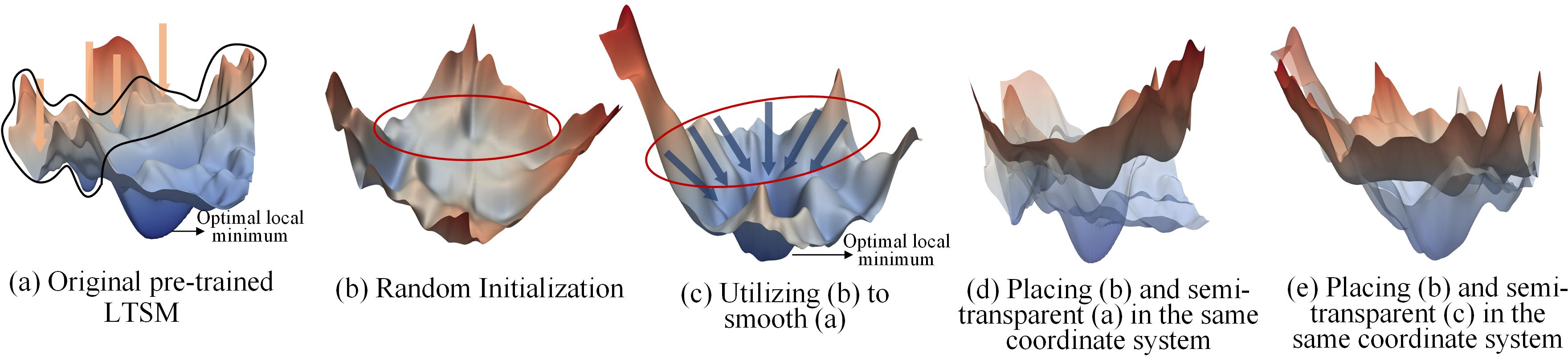
Figure 1: Loss landscape comparisons based on the LTSM Timer and exchange rate dataset. Smoother landscapes correspond to improved trainability; pre-trained weights (left) exhibit pronounced local protrusions and sharp minima.

Smoothed Full Fine-tuning (SFF): Methodology

The core contribution is a parameter-level weight interpolation algorithm, Smoothed Full Fine-tuning (SFF), which improves LTSM trainability by leveraging the complementary strengths of pre-trained and random weights. Specifically, SFF constructs an auxiliary LTSM via standard random initialization (Kaiming or Xavier), which exhibits a smooth and highly trainable loss landscape but lacks pre-trained temporal knowledge.

The smoothed model parameters are produced via linear interpolation:

$$\Theta_{\text{SFF}} = \alpha \Theta_{\text{pretrained}} + (1-\alpha)\Theta_{\text{random}}$$

where $\alpha \in (0,1)$ controls the tradeoff between preserved knowledge and smoothing. The resulting SFF weights retain pre-trained knowledge sufficient for strong zero-shot performance, while the overall energy landscape becomes significantly smoother, facilitating gradient-based optimization to superior generalizable minima during downstream fine-tuning.

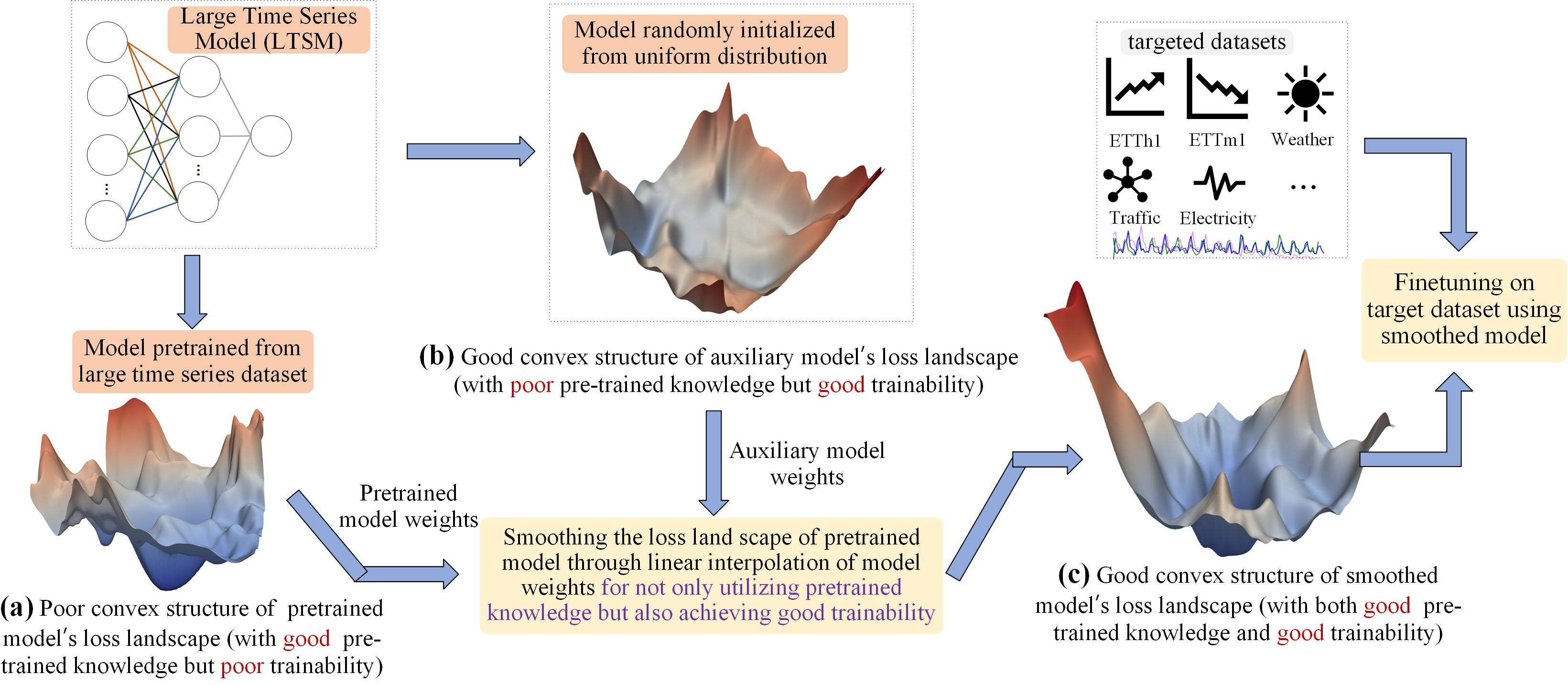
Figure 2: Smoothed Full Fine-tuning (SFF): a linear interpolation of pre-trained and random LTSM weights yields a smoother, more optimizable model with preserved temporal priors.

Theoretical Analysis: Landscape Smoothing and Minima Equilibria

A rigorous analysis decomposes the effects of SFF on sharp and flat minima. Sharpness is quantified as the maximum eigenvalue $\lambda_{\max}$ of the Hessian $\nabla^2\mathcal{L}(\Theta^*)$ at a local loss minimizer $\Theta^*$. Parameter perturbations (via interpolation) in sharp regions incur disproportionately large $\Delta\mathcal{L}$, while flat minima remain robust to such deviations. SFF's interpolation induces a convex combination of Hessians, reducing the local sharpness in high-curvature basins while flat regions remain unaltered:

$$\nabla^2 \mathcal{L}(\Theta_{\mathrm{SFF}}) \approx \alpha \nabla^2 \mathcal{L}(\Theta_{1}^{*}) + (1 - \alpha) \nabla^2 \mathcal{L}(\Theta_2)$$

Thus, $$\lambda_{\max}\bigl(\nabla^2\mathcal{L}(\Theta_{\mathrm{SFF}})\bigr) < \lambda_{\max}\bigl(\nabla^2\mathcal{L}(\Theta_{1}^{*})\bigr)$$ for suitable $\alpha$, directly smoothing out sharp minima and facilitating escape trajectories to broader, more generalizable attractors.

Moreover, the analysis demonstrates that standard random initializations (Kaiming/Xavier) yield flat loss landscapes, further supporting the choice of auxiliary models for landscape smoothing.

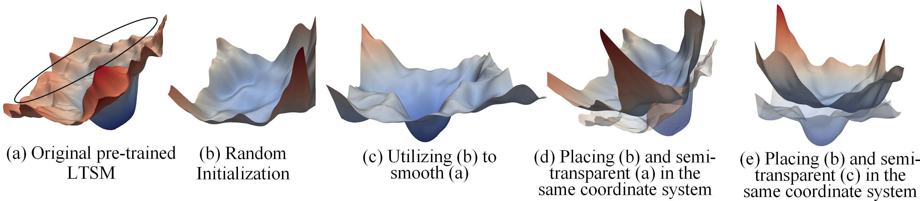
Figure 4: Loss landscape comparisons based on the LTSM Timer and weather dataset. Random initialization produces a much smoother and more convex surface than pre-training.

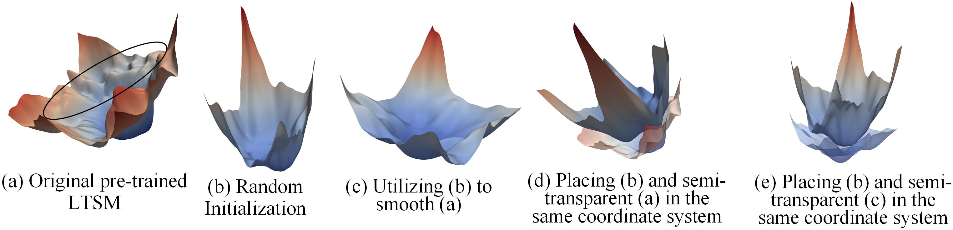
Figure 6: Loss landscape comparisons based on the LTSM Timer and electricity dataset—randomly initialized weights result in smoother, convex regions facilitating optimization.

Empirical Results: Time Series Forecasting, Anomaly Detection, and Imputation

SFF demonstrates consistent and robust improvements across multiple public datasets and LTSM architectures, including encoder-only (Moirai, MOMENT), decoder-only (Timer, TimesFM, Sundial), encoder-decoder (Chronos, UniTS), and MLP-only (TTMs). In multivariate time series forecasting with Timer, SFF achieves Mean Squared Error (MSE) reductions of 3–6.5% over direct full fine-tuning across different data proportions and consistently outperforms both training from scratch and strong baselines such as linear probing (LP), LP followed by FF (LPFF), LoRA, and popular regularization/optimization techniques including SAM, SWA, Mixout, and L2-SP.

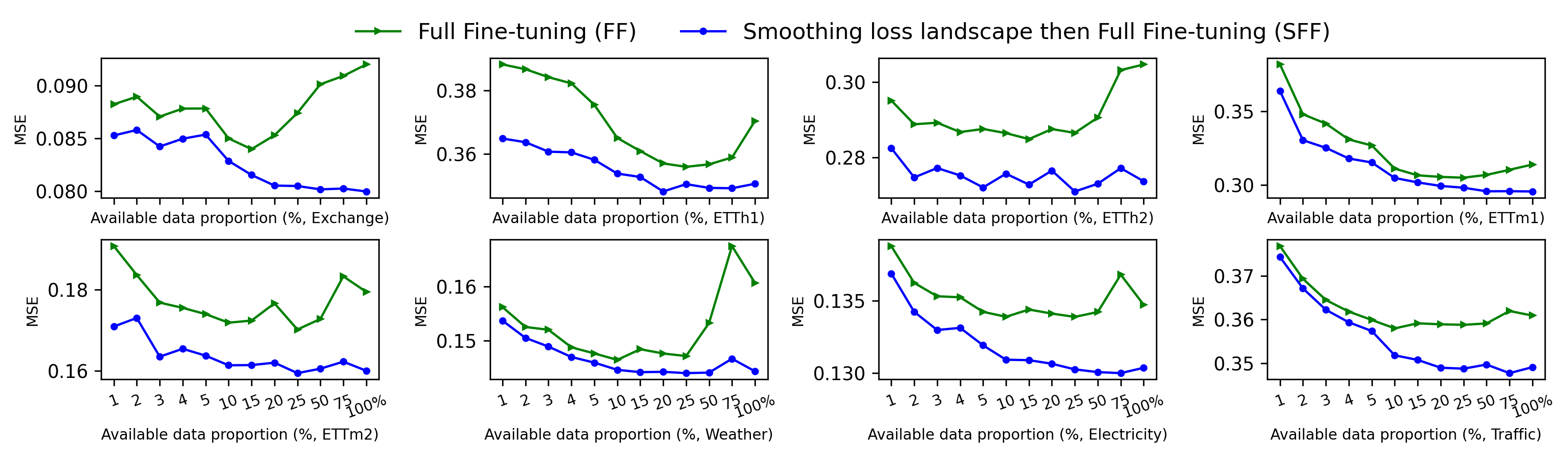
Figure 7: MSE of different fine-tuning strategies on Timer with prediction length 96, across datasets and data proportions. SFF achieves the lowest MSE at each regime.

Figure 8: Test MSE over epochs for different fine-tuning methods. SFF converges rapidly and to a lower error than standard fine-tuning, indicating retention of pre-trained knowledge and improved trainability.

SFF's smoothing operation also benefits zero-shot forecasting, with an average gain of 6.13% (Timer) and 35.75% (TimesFM). The interpolation coefficient $\alpha$ can be tuned for optimality, but SFF is robust to its setting, offering strong gains for $\alpha \in (0,1)$0 in a wide range.

Figure 3: Impact of interpolation coefficient $\alpha \in (0,1)$1 on zero-shot forecasting. SFF outperforms both pre-trained and randomly initialized extremes; $\alpha \in (0,1)$2 is optimal.

SFF provides improvements not only for forecasting but also for time series imputation and anomaly detection. In large-scale anomaly detection, SFF is the only method yielding higher anomaly segment MSE than both full fine-tuning and TFS, demonstrating substantive gains in out-of-distribution scenarios.

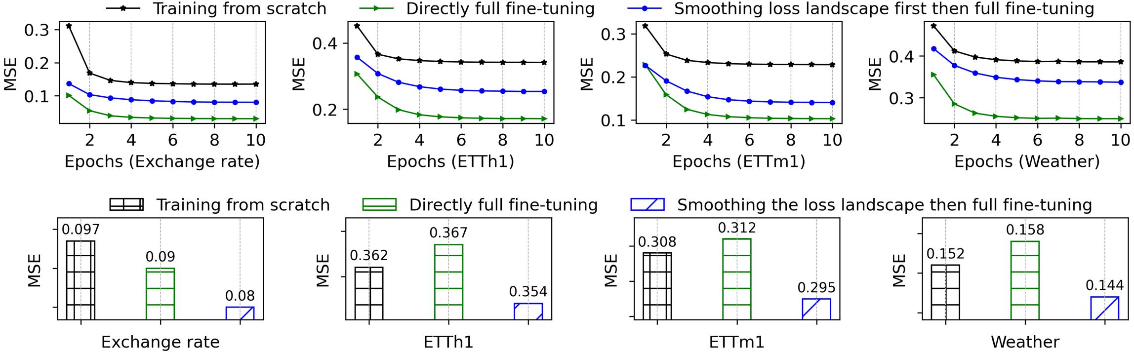
Figure 5: Training and testing losses for Timer: SFF (blue) achieves lower test loss and mitigates overfitting compared to FF (green) and TFS (black).

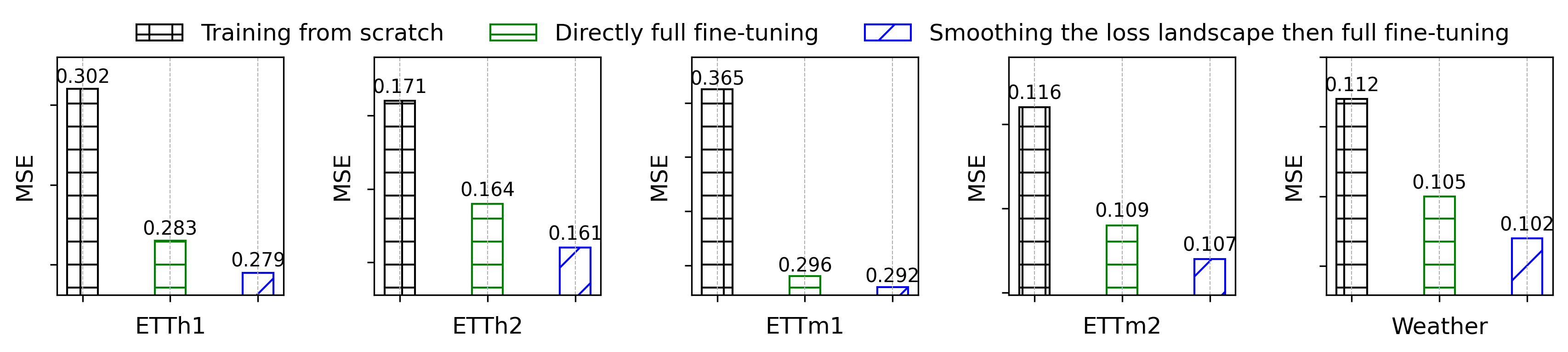
Figure 9: SFF consistently delivers lower imputation loss compared to FF and TFS at a 25% mask ratio.

Comparative Analysis and Robustness

SFF is superior not only to FF and TFS, but also to linear probing variants, LoRA, and other optimization approaches. The gains are particularly strong in the low-data regime and persist as the available fine-tuning data increases. The method is agnostic to network architecture, model scale (from 3.8 GB to 3 MB), LTSM design, or downstream time series task. Ablation shows the smoothing benefit is stable across Kaiming/Xavier initializations and is insensitive to initialization RNG seeds.

Practical and Theoretical Implications, Future Directions

The evidence demonstrates that overfitting during LTSM pretraining can result in pathological sharp minima, reducing downstream task performance and generalization. SFF offers a simple, memory- and compute-efficient mechanism to regularize the energy surface and unlock the representational capacity of LTSMs by explicitly addressing the loss landscape geometry issue at the parameter level.

Adopting SFF in LTSM fine-tuning pipelines is expected to become de facto best practice, enabling robust transfer of temporal representations across diverse domains. The methodology highlights a new frontier for foundation model adaptation: parameter-space perturbations designed via landscape geometry analysis. Extending this principle to other foundation models (e.g., vision, text, or graph domains) and developing meta-learned adaptive interpolation strategies for $\alpha \in (0,1)$3, or blockwise/local smoothing variants, are promising avenues.

Conclusion

The study establishes that direct fine-tuning of pre-trained LTSMs is fundamentally limited by the sharp, non-convex structure of their loss landscapes. SFF—parameter-space linear interpolation with random initializations—smooths these landscapes, preserving knowledge while enhancing trainability and generalization. Experimental results confirm the universality, consistency, and superiority of this approach across architectures, tasks, and data regimes, suggesting landscape smoothing as a critical ingredient for the next generation of efficient foundation model adaptation in time series and beyond.

Figure 10: Fine-tuning Timer for TSF, performance under different interpolation coefficients $\alpha \in (0,1)$4; larger $\alpha \in (0,1)$5 corresponds to greater retention of pre-trained knowledge, but moderate smoothing gives optimal test set performance.

(Figure 1–2, 7–10 referenced for landscape, empirical, and robustness analysis. See (2606.08578) for full details.)